Chapter 1 R Foundations
Meaningful data analysis requires the use of computer software.
R statistical software is one of the most popular tools for data analysis in academia, industry, and government. In what follows, I will attempt to lay a foundation of basic knowledge and skills with R that you will need for data analysis. I make no attempt to be exhaustive, and many other important aspects of using R (like plotting) will be discussed later, as needed.
1.1 Setting up R and RStudio Desktop
What is R?
R is a programming language and environment designed for statistical computing. It was introduced by Robert Gentleman and Robert Ihaka in 1993 as a free implementation of the S programming language developed at Bell Laboratories (https://www.r-project.org/about.html)
Some important facts about R are that:
- R is free, open source, and runs on many different types of computers (Windows, Mac, Linux, and others).
- R is an interactive programming language.
- You type and run a command in the Console for immediate feedback, in contrast to a compiled programming language, which compiles a program that is then executed.
- R is highly extendable.
- Many user-created packages are available to extend the functionality beyond what is installed by default.
- Users can write their own functions and easily add software libraries to R.
Installing R
To install R on your personal computer, you will need to download an installer program from the R Project’s website (https://www.r-project.org/). Links to download the installer program for your operating system should be found at https://cloud.r-project.org/. Click on the download link appropriate for your computer’s operating system and install R on your computer. If you have a Windows computer, a stable link for the most current installer program is available at https://cloud.r-project.org/bin/windows/base/release.html. (Similar links are not currently available for Mac and Linux computers.)
Installing RStudio
RStudio Desktop is a free “front end” for R provided by Posit Software (https://posit.co/). RStudio Desktop makes doing data analysis with R much easier by adding an Integrated Development Environment (IDE) and providing many other features. Currently, you may download RStudio at https://posit.co/download/rstudio-desktop/. You may need to navigate the RStudio website directly if this link no longer functions. Download the Free version of RStudio Desktop appropriate for your computer and install it.
Having installed both R and RStudio Desktop, you will want to open RStudio Desktop as you continue to learn about R.
RStudio Layout
RStudio Desktop has four panes:
- Console: the pane where commands are run.
- Source: the pane where you prepare commands to be run.
- Environment/History: the pane where you can see all the objects in your workspace, your command history, and other information.
- The Files/Plot/Packages/Help: the pane where you navigate between directories, where plots can be viewed, where you can see the packages available to be loaded, and where you can get help.
To see all RStudio panes, press the keys Ctrl + Alt + Shift + 0 on a PC or Cmd + Option + Shift + 0 on a Mac.
Figure 1.1 displays a labeled graphic of the panes. Your panes are likely in a different order than the graphic shown because I have customized my workspace for my own needs.
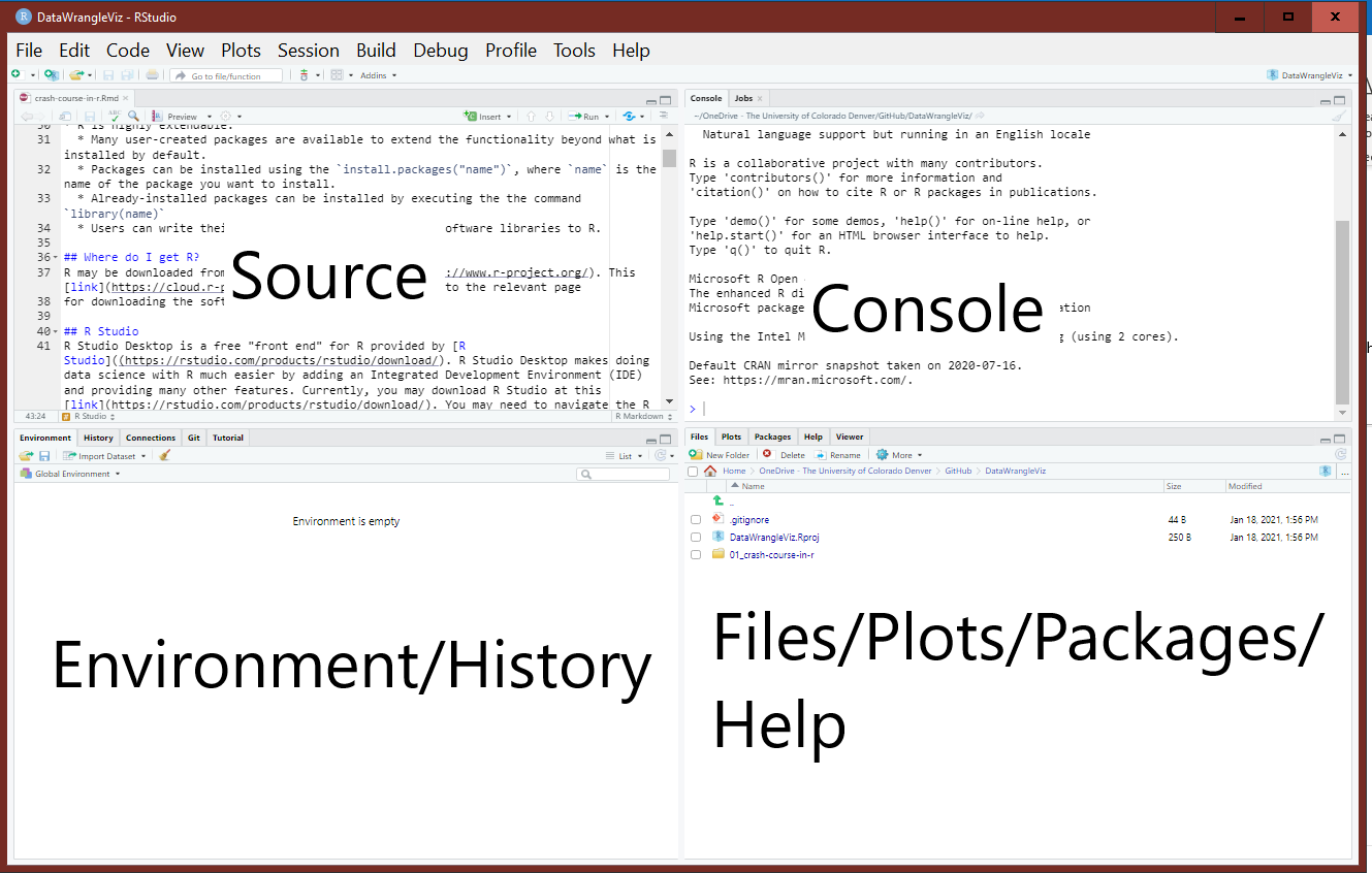
Figure 1.1: The RStudio panes labeled for convenience.
Customizing the RStudio workspace
At this point, I would highly encourage you to make one small workspace customization that will likely save you from experiencing future frustration. R provides a “feature” of that allows you to “save a workspace”. This allows you to easily pick up where you left off your last analysis. The issue with this is that over time you accumulate a lot of environmental artifacts that can conflict with each other. This can lead to errors and incorrect results that you will need to deal with. Additionally, this “feature” hinders the ability of others to reproduce your analysis because other users are unlikely to have the same workspace.
To turn off this feature, in the RStudio menu bar click Tools → Global Options and then make sure the “General” option is selected. Then make the following changes (if necessary):
- Uncheck the box for “Restore .RData into workspace at startup”.
- Change the toggle box for “Save workspace to .RData on exit” to “Never”.
- Click Apply then OK to save the changes.
Figure 1.2 displays what these options should look like.
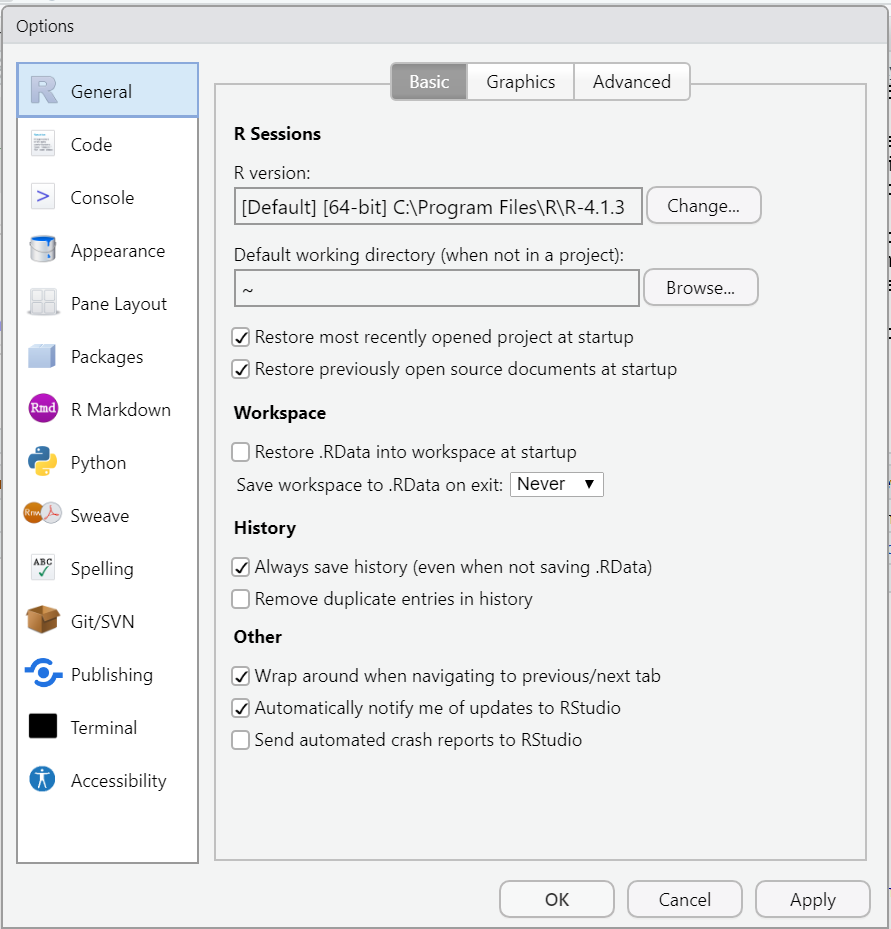
Figure 1.2: The General options window.
1.2 Running code, scripts, and comments
You can run code in R by typing it in the Console next to the > symbol and pressing the Enter key.
If you need to successively run multiple commands, it’s better to write your commands in a “script” file and then save the file. The commands in a Script file are often generically referred to as “code”.
Script files make it easy to:
- Reproduce your data analysis without retyping all your commands.
- Share your code with others.
A new Script file can be obtained by:
- Clicking File → New File → R Script in the RStudio menu bar.
- Pressing
Ctrl + Shift + non a PC orCmd + Shift + non a Mac.
There are various ways to run code from a Script file. The most common ones are:
- Highlight the code you want to run and click the Run button
 at the top of the Script pane.
 - Highlight the code you want to run and press “Ctrl + Enter” on your keyboard. If you don’t highlight anything, by default, RStudio runs the command the cursor currently lies on.
To save a Script file:
- Click File → Save in the RStudio menu bar.
- Press
Ctrl + son a PC orCmd + son a Mac.
A comment is a set of text ignored by R when submitted to the Console.
A comment is indicated by the # symbol. Nothing to the right of the # is executed by the Console.
To comment (or uncomment) multiple lines of code in the Source pane of RStudio, highlight the code you want to comment and press Ctrl + Shift + c on a PC or Cmd + Shift + c on a Mac.
Your turn
Perform the following tasks:
- Type
1+1in the Console and press Enter. - Open a new Script in RStudio.
- Type
mean(1:3)in your Script file. - Type
# mean(1:3)in your Script file. - Run the commands from the Script using an approach mentioned above.
- Save your Script file.
- Use the keyboard shortcut to “comment out” some of the lines of your Script file.
1.3 Assignment
R works on various types of objects that we’ll learn more about later.
To store an object in the computer’s memory we must assign it a name using the assignment operator <- or the equal sign =.
Some comments:
- In general, both
<-and=can be used for assignment. - Pressing
Alt + -on a PC orOption + -on a Mac will insert<-into the R Console and Script files.- If you are creating an R Markdown file, then this shortcut will only insert
<-if you are in an R code block.
- If you are creating an R Markdown file, then this shortcut will only insert
<-and=are NOT synonyms, but can be used identically most of the time.
It is best to use <- for assigning a name to an object and reserving = for specifying function arguments. See Section 1.14.1 for an explanation.
Once an object has been assigned a name, it can be printed by running the name of the object in the Console or using the print function.
Your turn
Run the following commands in the Console:
# compute the mean of 1, 2, ..., 10 and assign the name m
m <- mean(1:10)
m # print m
print(m) # print m a different way
After the comment, we compute the sample mean of the values \(1, 2, \ldots, 10\), then assign it the name m. The next two lines are different mechanisms for printing the information contained in the object m (which is just the number 5.5).
1.4 Functions
A function is an object that performs a certain action or set of actions based on objects it receives from its arguments. We use a sequence of function calls to perform data analysis.
To use a function, you type the function’s name in the Console (or Script) and then supply the function’s “arguments” between parentheses, ().
The arguments of a function are pieces of data or information the function needs to perform the requested task (i.e., the function “inputs”). Each argument you supply is separated by a comma, ,. Some functions have default values for certain arguments and do not need to specified unless something beside the default behavior is desired.
e.g., the mean function computes the sample mean of an R object x. (How do I know? Because I looked at the documentation for the function by running ?mean in the Console. We’ll talk more about getting help with R shortly.) The mean function also has a trim argument that indicates the, “… fraction … of observations to be trimmed from each end of x before the mean is computed” (R Core Team (2024), ?mean).
Consider the examples below, in which we compute the mean of the set of values 1, 5, 3, 2, 10.
The output differs for the two function calls because in the first we compute (1 + 5 + 3 + 4 + 10)/5 = 23/5 = 4.6 while in the second we remove the first 20% and last 20% of the values (i.e., dropping 1 and 10) and compute (5 + 3 + 4)/3 = 12/3 = 4.
1.5 Packages
Packages are collections of functions, data, and other objects that extend the functionality available in R by default.
R packages can be installed using the install.packages function and loaded using the library function.
Your turn
The tidyverse (https://www.tidyverse.org, Wickham (2023c)) is a popular ecosystem of R packages used for manipulating, tidying, and plotting data. Currently, the tidyverse is comprised of the following packages:
- ggplot2: A package for plotting based on the “Grammar of Graphics” (Wickham et al. 2024).
- purrr: A package for functional programming (Wickham and Henry 2023).
- tibble: A package providing a more advanced data frame (Müller and Wickham 2023).
- dplyr: A package for manipulating data. More specifically, it provides ” a grammar of data manipulation” (Wickham et al. 2023).
- tidyr: A package to help create “tidy” data (Wickham, Vaughan, and Girlich 2024). Tidy data is an data organization style often convenient for data analysis.
- stringr: A package for working with character/string data (Wickham 2023b).
- readr: A package for importing data (Wickham, Hester, and Bryan 2024).
- forcats: A package for working with categorical data (Wickham 2023a).
Install the set of tidyverse R packages by running the command below in the Console.
After you install tidyverse, load the package(s) by running the command below.
You should see something like the following output:
## ── Attaching core tidyverse packages ────────────────────────────────── tidyverse 2.0.0 ──
## ✔ dplyr     1.1.4     ✔ readr     2.1.5
## ✔ forcats   1.0.0     ✔ stringr   1.5.1
## ✔ ggplot2   3.5.1     ✔ tibble    3.2.1
## ✔ lubridate 1.9.3     ✔ tidyr     1.3.1
## ✔ purrr     1.0.2
## ── Conflicts ──────────────────────────────────────────────────── tidyverse_conflicts() ──
## ✖ dplyr::filter() masks stats::filter()
## ✖ dplyr::lag()    masks stats::lag()
## ℹ Use the conflicted package (<http://conflicted.r-lib.org/>) to force all conflicts to become errors
Different packages may use the same function name to provide certain functionality. The functions will likely be used for different tasks or require different arguments. E.g., You may have noticed when you loaded the tidyverse above that dplyr::lag() masks stats::lag(). What this means is that both the dplyr and stats packages have a function called lag.
To refer to a function in a specific package, we should add package:: prior to the function name. In the code below, we run stats::lag and dplyr::lag on two different objects using the :: syntax.
stats::lag(1:10, 2)
##  [1]  1  2  3  4  5  6  7  8  9 10
## attr(,"tsp")
## [1] -1  8  1
dplyr::lag(1:10, 2)
##  [1] NA NA  1  2  3  4  5  6  7  8
The output returned by the two functions is different because the functions are intended to do different things. The stats::lag function call shifts the time base of the provided time series object back 2 units, while the call to dplyr::lag provides the values 2 positions earlier in the object. Note: you don’t need to understand the lag function in the example above. The example is provided to demonstrate how to use the :: syntax to call to a function in a specific package when the function name has conflicts in multiple packages.
1.6 Getting help
There are many ways to get help in R.
If you know the command for which you want help, then run ?command (where command is replaced the name of the relevant command) in the Console, to access the documentation for the object. This approach will also work with data sets, package names, object classes, etc. If you need to refer to a function in a specific package, you can use ?package::function to get help on a specific function, e.g., ?dplyr::filter.
The documentation will provide:
- A Description section with general information about the function or object.
- A **Usage* section with a generic template for using the function or object.
- An Arguments section summarizing the function inputs the function needs.
- A Details section may be provided with additional information about how the function or object.
- A Value section that describes what is returned by the function.
- A Examples section providing examples of how to use the function. Usually, these can be copied and pasted into the Console to better understand the function arguments and what it produced.
If you need to find a command to help you with a certain topic, then ??topic will search for the topic through all installed documentation and bring up any vignettes, code demonstrations, or help pages that include the topic for which you searched.
If you are trying to figure out why an error is being produced, what packages can be used to perform a certain analysis, how to perform a complex task that you can’t seem to figure out, etc., then simply do a web search for what you’re trying to figure out! Because R is such a popular programming language, it is likely you will find a stackoverflow response, a helpful blog post, an R users forum response, etc., that at least partially addresses your question.
Do the following:
- Run
?lmin the Console to get help on thelmfunction, which is one of the main functions used for fitting linear models. - Run
??logarithmsin the Console to search the R documentation for information about logarithms. It is likely that you will see multiple Help pages that mention “logarithm”, so you may end up needing to find the desired entry via trial and error. - Run a web search for something along the lines of “How do I change the size of the axis labels in an R plot?”.
1.7 Data types and structures
1.7.1 Basic data types
R has 6 basic (“atomic”) vector types (https://cran.r-project.org/doc/manuals/r-release/R-lang.html#Basic-types) (R Core Team 2024):
- character: collections of characters. E.g.,
"a","hello world!". - double: decimal numbers. e.g.,
1.2,1.0. - integer: whole numbers. In R, you must add
Lto the end of a number to specify it as an integer. E.g.,1Lis an integer but1is a double. - logical: boolean values,
TRUEandFALSE. - complex: complex numbers. E.g.,
1+3i. - raw: a type to hold raw bytes.
Both double and integer values are specific types of numeric values.
The typeof function returns the R internal type or storage mode of any object.
Consider the following commands and output:
1.7.2 Other important object types
There are other important types of objects in R that are not basic. We will discuss a few. The R Project manual provides additional information about available types (https://cran.r-project.org/doc/manuals/r-release/R-lang.html#Basic-types).
1.7.2.1 Numeric
An object is numeric if it is of type integer or double. In that case, it’s mode is said to be numeric.
The is.numeric function tests whether an object can be interpreted as numbers. We can use it to determine whether an object is numeric, as in the code run below.
1.7.2.2 NULL
NULL is a special object to indicate an object is absent. An object having a length of zero is not the same thing as an object being absent.
1.7.3 Data structures
R operates on data structures. A data structure is a “container” that holds certain kinds of information.
R has 5 basic data structures:
- vector.
- matrix.
- array.
- data frame.
- list.
Vectors, matrices, and arrays are homogeneous objects that can only store a single data type at a time. Data frames and lists can store multiple data types.
Vectors and lists are considered one-dimensional objects. A list is technically a vector. Vectors of a single type are atomic vectors (https://cran.r-project.org/doc/manuals/r-release/R-lang.html#List-objects). Matrices and data frames are considered two-dimensional objects. Arrays can have 1 or more dimensions.
The relationship between dimensionality and data type for the basic data structures is summarized in Table 1.1, which is based on a table in the first edition of Hadley Wickham’s Advanced R (https://adv-r.had.co.nz/Data-structures.html#data-structure).
| # of dimensions | homogeneous data | heterogeneous data |
|---|---|---|
| 1 | atomic vector | list |
| 2 | matrix | data frame |
| 1 or more | array |
1.8 Vectors
A vector is a one-dimensional set of data of the same type.
1.8.1 Creation
The most basic way to create a vector is the c (combine) function. The c function combines values into an atomic vector or list.
The following commands create vectors of type numeric, character, and logical, respectively.
c(1, 2, 5.3, 6, -2, 4)c("one", "two", "three")c(TRUE, TRUE, FALSE, TRUE)
R provides two main functions for creating vectors with specific patterns: seq and rep.
The seq (sequence) function is used to create an equidistant series of numeric values. Some examples:
seq(1, 10)creates a sequence of numbers from 1 to 10 in increments of 1.1:10creates a sequence of numbers from 1 to 10 in increments of 1.seq(1, 20, by = 2)creates a sequence of numbers from 1 to 20 in increments of 2.seq(10, 20, len = 100)creates a sequence of numbers from 10 to 20 of length 100.
The rep (replicate) function can be used to create a vector by replicating values. Some examples:
rep(1:3, times = 3)replicates the sequence1, 2, 3three times in a row.rep(c("trt1", "trt2", "trt3"), times = 1:3)replicates"trt1"once,"trt2"twice, and"trt3"three times.rep(1:3, each = 3)replicates each element of the sequence 1, 2, 3 three times.
Multiple vectors can be combined into a new vector object using the c function. E.g., c(v1, v2, v3) would combine vectors v1, v2, and v3.
Your turn
Run the commands below in the Console to see what is printed. After you do that, try to answer the following questions:
- What does the
byargument of theseqfunction control? - What does the
lenargument of theseqfunction control? - What does the
timesargument of therepfunction control? - What does the
eachargument of therepfunction control?
# vector creation
c(1, 2, 5.3, 6, -2, 4)
c("one", "two", "three")
c(TRUE, TRUE, FALSE, TRUE)
# sequences of values
seq(1, 10)
1:10
seq(1, 20, by = 2)
seq(10, 20, len = 100)
# replicated values
rep(1:3, times = 3)
rep(c("trt1", "trt2", "trt3"), times = 1:3)
rep(1:3, each = 3)
Next, we can practice combining multiple vectors using c. Run the commands below in the Console.
1.8.2 Categorical vectors
Categorical data should be stored as a factor in R. Even though your code related to categorical data may work when stored as character or numeric data because a cautious developer planned for that possibility, it is best to use good coding practices that minimize potential issues.
The factor function takes a vector of values that can be coerced to type character and converts them to an object of class factor. In the code chunk below, we create two factor objects from vectors.
# create some factor variables
f1 <- factor(rep(1:6, times = 3))
f1
##  [1] 1 2 3 4 5 6 1 2 3 4 5 6 1 2 3 4 5 6
## Levels: 1 2 3 4 5 6
f2 <- factor(c("a", 7, "blue", "blue", FALSE))
f2
## [1] a     7     blue  blue  FALSE
## Levels: 7 a blue FALSE
Note that when a factor object is printed that it lists the Levels (i.e., unique categories) of the object.
Some additional comments:
factorobjects aren’t technically vectors (e.g., runningis.factor(f2)based on the above code will returnFALSE) though they essentially behave like vectors, which is why they are included here.- The
is.factorfunction can be used to determine whether an object is afactor. - You can create
factorobjects with specific orderings of categories using thelevelandorderedarguments of thefactorfunction (see?factorfor more details).
Your turn
Attempt to complete the following tasks:
- Create a vector named
grpthat has two levels:aandb, where the first 7 values areaand the second 4 values areb. - Run
is.factor(grp)in the Console. - Run
is.vector(grp)in the Console. - Run
typeof(grp)in the Console.
Related to the last task, a factor object is technically a collection of integers that have labels associated with each unique integer value.
Let’s look at creating ordered factor objects. Suppose we have categorical data with the categories small, medium, and large. We create a size vector with hypothetical data below.
If we convert size to a factor, R will automatically order the levels of size alphabetically.
This is not technically a problem, but can result in undesirable side effects such as plots with levels in an undesirable order.
To create an ordered vector, we specify the desired order of the levels and set the ordered argument to TRUE, as in the code below.
1.8.3 Extracting parts of a vector
Parts a vector can be extracted by appending an index vector in square brackets [] to the name of the vector, where the index vector indicates which parts of the vector to retain or exclude. We can include either numbers or logical values in our index vector. We discuss both approaches below.
1.8.3.1 Selection use a numeric index vector
Let’s create a numeric vector a with the values 2, 4, 6, 8, 10, 12, 14, 16.
To extract the 2nd, 4th, and 6th elements of a, we can use the code below. The code indicates that the 2nd, 4th, and 6th elements of a should be extracted.
You can also use “negative” indexing to indicate the elements of the vector you want to exclude. Specifically, supplying a negative index vector indicates the values you want to exclude from your selection.
In the example below, we use the minus (-) sign in front of the index vector c(2, 4, 6) to indicate we want all elements of a EXCEPT the 2nd, 4th, and 6th. The last line of code excludes the 3rd through 6th elements of a.
1.8.3.2 Logical expressions
A logical expression uses one or more logical operators to determine which elements of an object satisfy the specified statement. The basic logical operators are:
<,<=: less than, less than or equal to.>,>=: greater than, greater than or equal to.==: equal to.!=: not equal to.
Creating a logical expression with a vector will result in a logical vector indicating whether each element satisfies the logical expression.
Your turn
Run the following commands in R and see what is printed. What task is each statement performing?
We can create more complicated logical expressions using the “and”, “or”, and “not” operators.
&: and.|: or.!: not, i.e., not true.
The & operator returns TRUE if all logical values connected by the & are TRUE, otherwise it returns FALSE. On the other hand, the | operator returns TRUE if any logical values connected by the | are TRUE, otherwise it returns FALSE. The ! operator returns the complement of a logical value or expression.
Your turn
Run the following commands below in the Console.
What role does & serve in a sequence of logical values? Similarly, what roles do | and ! serve in a sequence of logical values?
Logical expressions can be connected via & and | (and impacted via !), in which case the operators are applied elementwise (i.e., to all of the first elements in the expressions, then all the second elements in the expressions, etc).
Your turn
Run the following commands in R and see what is printed. What task is each statement performing? Note that the parentheses () are used to group logical expressions to more easily understand what is being done. This is a good coding style to follow.
1.8.3.3 Selection using logical expressions
Logical expressions can be used to return parts of an object satisfying the appropriate criteria. Specifically, we pass logical expressions within the square brackets to access part of a data structure. This syntax will return each element of the object for which the expression is TRUE.
1.9 Helpful functions
We provide a brief overview of R functions we often use in our data analysis.
1.9.1 General functions
For brevity, Table 1.2 provides a table of functions commonly useful for basic data analysis along with a description of their purpose.
| function | purpose |
|---|---|
length |
Determines the length/number of elements in an object. |
sum |
Sums the elements in the object. |
mean |
Computes the sample mean of the elements in an object. |
var |
Computes the sample variance of the elements in an object. |
sd |
Computes the sample standard deviation the elements of an object. |
range |
Determines the range (minimum and maximum) of the elements of an object. |
log |
Computes the (natural) logarithm of elements in an object. |
summary |
Returns a summary of an object. The output changes depending on the class type of the object. |
str |
Provides information about the structure of an object. Usually, the class of the object and some information about its size. |
Your turn
Run the following commands in the Console. Determine for yourself what task each command is performing.
# common functions
x <- rexp(100) # sample 100 iid values from an Exponential(1) distribution
length(x) # length of x
sum(x) # sum of x
mean(x) # sample mean of x
var(x) # sample variance of x
sd(x) # sample standard deviation of x
range(x) # range of x
log(x) # logarithm of x
summary(x) # summary of x
str(x) # structure of x1.10 Data Frames
Data frames are two-dimensional data objects. Each column of a data frame is a vector (or variable) of possibly different data types. This is a fundamental data structure used by most of R’s modeling software. The class of a base R data frame is data.frame, which is technically a specially structured list.
In general, I recommend tidy data, which means that each variable forms a column of the data frame, and each observation forms a row.
1.10.1 Direct creation
Data frames are directly created by passing vectors into the data.frame function.
The names of the columns in the data frame are the names of the vectors you give the data.frame function. Consider the following simple example.
# create basic data frame
d <- c(1, 2, 3, 4)
e <- c("red", "white", "blue", NA)
f <- c(TRUE, TRUE, TRUE, FALSE)
df <- data.frame(d,e,f)
df
##   d     e     f
## 1 1   red  TRUE
## 2 2 white  TRUE
## 3 3  blue  TRUE
## 4 4  <NA> FALSE
The columns of a data frame can be renamed using the names function on the data frame and assigning a vector of names to the data frame.
# name columns of data frame
names(df) <- c("ID", "Color", "Passed")
df
##   ID Color Passed
## 1  1   red   TRUE
## 2  2 white   TRUE
## 3  3  blue   TRUE
## 4  4  <NA>  FALSE
The columns of a data frame can be named when you are first creating the data frame by using name = for each vector of data.
1.10.2 Importing Data
Direct creation of data frames is only appropriate for very small data sets. In practice, you are likely to have a file that contains the data you want to analyze and you want to import the data into R.
The read.table function imports data in table format from file into R as a data frame.
The basic usage of this function is: read.table(file, header = TRUE, sep = ",")
fileis the file path and name of the file you want to import into R.- If you don’t know the file path, setting
file = file.choose()will bring up a dialog box asking you to locate the file you want to import.
- If you don’t know the file path, setting
headerspecifies whether the data file has a header (variable labels for each column of data in the first row of the data file).- If you don’t specify this option in R or use
header = FALSE, then R will assume the file doesn’t have any headings. header = TRUEtells R to read in the data as a data frame with column names taken from the first row of the data file.
- If you don’t specify this option in R or use
sepspecifies the delimiter separating elements in the file.- If each column of data in the file is separated by a space, then use
sep = " ". - If each column of data in the file is separated by a comma, then use
sep = ",". - If each column of data in the file is separated by a tab, then use
sep = "\t".
- If each column of data in the file is separated by a space, then use
Your turn
Consider reading in a csv (comma separated file) with a header. The file in question contains information related to COVID-19 cases and deaths as of February 4, 2021. The file is available on the internet in the author’s GitHub repository. Notice that we specify the path of the file (https://raw.githubusercontent.com/jfrench/DataWrangleViz/master/data/) prior to specifying the file name (covid_dec4.csv). Since the file has a header, we specify header = TRUE. Since the data values are separated by commas, we specify sep = ",". Run the code below in your R Console.
# import data as data frame
dtf <- read.table(file = "https://raw.githubusercontent.com/jfrench/DataWrangleViz/master/data/covid_dec4.csv",
                  header = TRUE,
                  sep = ",")
str(dtf)
## 'data.frame':    50 obs. of  7 variables:
##  $ state_name: chr  "Alabama" "Alaska" "Arizona" "Arkansas" ...
##  $ state_abb : chr  "AL" "AK" "AZ" "AR" ...
##  $ deaths    : int  3831 142 6885 2586 19582 2724 5146 782 19236 9725 ...
##  $ population: num  387000 96500 498000 238000 2815000 ...
##  $ income    : int  25734 35455 29348 25359 31086 35053 37299 32928 27107 28838 ...
##  $ hs        : num  82.1 91 85.6 82.9 80.7 89.7 88.6 87.7 85.5 84.3 ...
##  $ bs        : num  21.9 27.9 25.9 19.5 30.1 36.4 35.5 27.8 25.8 27.3 ...
Running str on the data frame gives us a general picture of the values stored in the data frame.
Note that the read_table function in the readr package (Wickham, Hester, and Bryan 2024) is perhaps a better way of reading in tabular data and uses similar syntax. To import data contained in Microsoft Excel files, you can use functions available in the readxl package (Wickham and Bryan 2023).
1.10.3 Extracting parts of a data frame
R provides many ways to extract parts of a data frame. We will provide several examples using the mtcars data frame in the datasets package.
The mtcars data frame 32 observations of 11 variables. The variables are:
mpg: miles per gallon.cyl: number of cylinders.disp: engine displacement (cubic inches).hp: horsepower.drat: rear axle ratio.wt: weight in 1000s of pounds.qsec: time in seconds to travel 0.25 of a mile.vs: engine shape (0 = V-shaped, 1 = straight).am: transmission type (0 = automatic, 1 = manual).gear: number of forward gears.carb: number of carburetors.
We load the data set and examine the basic structure by running the commands below.
data(mtcars) # load data set
str(mtcars)  # examine data structure
## 'data.frame':    32 obs. of  11 variables:
##  $ mpg : num  21 21 22.8 21.4 18.7 18.1 14.3 24.4 22.8 19.2 ...
##  $ cyl : num  6 6 4 6 8 6 8 4 4 6 ...
##  $ disp: num  160 160 108 258 360 ...
##  $ hp  : num  110 110 93 110 175 105 245 62 95 123 ...
##  $ drat: num  3.9 3.9 3.85 3.08 3.15 2.76 3.21 3.69 3.92 3.92 ...
##  $ wt  : num  2.62 2.88 2.32 3.21 3.44 ...
##  $ qsec: num  16.5 17 18.6 19.4 17 ...
##  $ vs  : num  0 0 1 1 0 1 0 1 1 1 ...
##  $ am  : num  1 1 1 0 0 0 0 0 0 0 ...
##  $ gear: num  4 4 4 3 3 3 3 4 4 4 ...
##  $ carb: num  4 4 1 1 2 1 4 2 2 4 ...
We should do some data cleaning on this data set (see Chapter 2), but we will refrain from this for simplicity.
1.10.3.1 Direct extraction
The column variables of a data frame may be extracted from a data frame by specifying the data frame’s name, then $, and then specifying the name of the desired variable. This pulls the actual variable vector out of the data frame, so the thing extracted is a vector, not a data frame.
Below, we extract the mpg variable from the mtcars data frame.
mtcars$mpg
##  [1] 21.0 21.0 22.8 21.4 18.7 18.1 14.3 24.4 22.8 19.2 17.8 16.4 17.3 15.2 10.4
## [16] 10.4 14.7 32.4 30.4 33.9 21.5 15.5 15.2 13.3 19.2 27.3 26.0 30.4 15.8 19.7
## [31] 15.0 21.4
Another way to extract a variable from a data frame as a vector is df[, "var"], where df is the name of our data frame and var is the desired variable name. This syntax uses a df[rows, columns] style syntax, where rows and columns indicate the desired rows or columns. If either the rows or columns are left blank, then all rows or columns, respectively, are extracted.
mtcars[,"mpg"]
##  [1] 21.0 21.0 22.8 21.4 18.7 18.1 14.3 24.4 22.8 19.2 17.8 16.4 17.3 15.2 10.4
## [16] 10.4 14.7 32.4 30.4 33.9 21.5 15.5 15.2 13.3 19.2 27.3 26.0 30.4 15.8 19.7
## [31] 15.0 21.4
Once again, this action returns a vector, not a data frame. The is because the [ operator has an argument drop that is set to TRUE by default by when using [rows, columns] style extraction. The drop argument controls whether the result is coerced to the lowest possible dimension.
To get around this behavior we can change the drop argument to FALSE, as shown below (some output suppressed).
# extract mpg variable, keep as data frame
mtcars[,"mpg", drop = FALSE]
##                      mpg
## Mazda RX4           21.0
## Mazda RX4 Wag       21.0
## Datsun 710          22.8
....
An easier approach to avoid the default drop behavior is the slightly different syntax df["var"] (notice we no longer have the comma to separate rows and columns). We use this syntax below, suppressing part of the output, for the mpg variable in mtcars.
# extract mpg variable, keep as data frame
mtcars["mpg"]
##                      mpg
## Mazda RX4           21.0
## Mazda RX4 Wag       21.0
## Datsun 710          22.8
....
To select multiple variables in a data frame, we can provide a character vector with multiple variable names between []. In the example below, we extract both the mpg and cyl variables from mtcars.
mtcars[c("mpg", "cyl")]
##                      mpg cyl
## Mazda RX4           21.0   6
## Mazda RX4 Wag       21.0   6
## Datsun 710          22.8   4
....
You can also use numeric indices to directly indicate the rows or columns of the data frame that you would like to extract. Alternatively, you can use variable names for the columns.
df[1,]would access the first row ofdf.df[1:2,]would access the first two rows ofdf.df[,2]would access the second column ofdf.df[1:2, 2:3]would access the information in rows 1 and 2 of columns 2 and 3 ofdf.df[c(1, 3, 5), c("var1", "var2")]would access the information in rows 1, 3, and 5 of thevar1andvar2variables.
We practice these techniques below.
Run the following commands in the Console. Determine what task each command is performing.
# Extract parts of a data frame
df3 <- data.frame(numbers = 1:5,
                  characters = letters[1:5],
                  logicals = c(TRUE, TRUE, FALSE, TRUE, FALSE))
df3 # print df3
df3$logicals # extract the logicals vector of df3
df3[1, ] # extract the first column of df3
df3[, 3] # extract the third column of df3
df3[, 2:3] # extract column 2 and 3 of df3
# extract the numbers and logical columns of df3
df3[, c("numbers", "logicals")]
df3[c("numbers", "logicals")]
1.10.3.2 Extraction using logical expressions
Logical expressions can be used to subset a data frame.
To select specific rows of a data frame, we use the syntax df[logical vector, ], where logical vector is a valid logical vector whose length matches the number of rows in the data frame. Usually, the logical vector is created using a logical expression involving one or more data frame variables. In the code below, we extract the rows of the mtcars data frame for which the hp variable is more than 250.
# extract rows with hp > 250
mtcars[mtcars$hp > 250,]
##                 mpg cyl disp  hp drat   wt qsec vs am gear carb
## Ford Pantera L 15.8   8  351 264 4.22 3.17 14.5  0  1    5    4
## Maserati Bora  15.0   8  301 335 3.54 3.57 14.6  0  1    5    8
We can make the logical expression more complicated and also select specific variables using the syntax discussed in Section 1.10.3.1. Below, we extract the rows of mtcars with 8 cylinders and mpg > 17, while extracting only the mpg, cyl, disp, and hp variables.
1.10.3.3 Extraction using the subset function
The techniques for extracting parts of a data frame discussed in Sections 1.10.3.1 and 1.10.3.2 are the fundamental approaches for selecting desired parts of a data frame. However, these techniques can seem complex and difficult to interpret, particularly when looking back at code you have written in the past. A sleeker approach to extracting part of a data frame is to use the subset function.
The subset function returns the part of a data frame that meets the specified conditions. The basic usage of this function is: subset(x, subset, select, drop = FALSE)
xis the object you want to subset.xcan be a vector, matrix, or data frame.
subsetis a logical expression that indicates the elements or rows ofxto keep (TRUEmeans keep).selectis a vector that indicates the columns to keep.dropis a logical value indicating whether the data frame should “drop” into a vector if only a single row or column is kept. The default isFALSE, meaning that a data frame will always be returned by thesubsetfunction by default.
There are many clever ways of using subset to select specific parts of a data frame. We encourage the reader to run ?base::subset in the Console for more details.
Your turn
Run the following commands in the Console to use the subset function to extract parts of the mtcars data frame.
subset(mtcars, subset = gear > 4). This command will subset the rows ofmtcarsthat have more than 4 gears. Note any variables referred to in thesubsetfunction are assumed to be part of the supplied data frame or are available in memory.subset(mtcars, select = c(disp, hp, gear)). This command will select thedisp,hp, andgearvariables ofmtcarsbut will exclude the other columns.subset(mtcars, subset = gear > 4, select = c(disp, hp, gear))combines the previous two subsets into a single command.
An advantage of the subset function is that it makes code easily readable. This is important for collaborating with others, including your future self! Using base R, the final code example above would be: mtcars[mtcars$gear>4, c("disp", "hp", "gear")]
It is difficult to look at base R code and immediately tell what it happening, so the subset function adds clarity.
1.11 Using the pipe operator
R’s native pipe operator (|>) allows you to “pipe” the object on the left side of the operator into the first argument of the function on the right side of the operator. There are ways to modify this default behavior, but we will not discuss them.
The pipe operator is a convenient way to string together numerous steps in a string of commands. This coding style is generally considered more readable than other approaches because you can incrementally modify the object through each pipe and each step of the pipe is easy to understand. Ultimately, it’s a stylistic choice that can decide to adopt or ignore.
Consider the following approaches to extracting part of mtcars. We choose the rows for which engine displacement is more than 400 and only keep the mpg, disp, and hp columns. We can do this in a single function call, but the piping approach breaks the action into smaller parts.
# two styles for select certain rows and columns of mtcars
subset(mtcars,
       subset = disp > 400,
       select = c(mpg, disp, hp))
##                      mpg disp  hp
## Cadillac Fleetwood  10.4  472 205
## Lincoln Continental 10.4  460 215
## Chrysler Imperial   14.7  440 230
mtcars |>
  subset(subset = disp > 400) |>
  subset(select = c(mpg, disp, hp))
##                      mpg disp  hp
## Cadillac Fleetwood  10.4  472 205
## Lincoln Continental 10.4  460 215
## Chrysler Imperial   14.7  440 230
When reading code with pipes, the pipe can be thought of as the word “then”. In the code above, we take mtcars then subset it based on disp and then select some columns.
Most parts of the world do not use miles per gallon to measure fuel economy because they don’t measure distance in miles nor volume in gallons. A common measure of fuel economy is the liters of fuel required to travel 100 kilometers. Noting that 3.8 liters is (approximately) equivalent to 1 (U.S.) gallon and 1.6 kilometers is (approxiomately) equivalent to 1 mile, we can convert fuel economy of \(x\) miles per gallon to liters per 100 kilometers by noting:
\[\frac{1}{x}\frac{\mathrm{gal}}{\mathrm{mi}}\times\frac{3.8}{1}\frac{\mathrm{L}}{\mathrm{gal}}\times\frac{1}{1.6}\frac{\mathrm{mi}}{\mathrm{km}}\times\frac{100\;\mathrm{km}}{100\;\mathrm{km}} = \frac{237.5}{x}\frac{\mathrm{L}}{100\;\mathrm{km}}.\]
Thus, to convert from miles per gallon to liters per 100 kilometers, we take 237.5 and divide by the number of miles per gallon.
In the next set of code, we create a new variable, lp100km, in the mtcars data frame that describes the liters of fuel each car requires to travel 100 kilometers. Then we select only the columns mpg and lp100km. We then look at only the first 5 observations. To create the new variable, lp100km, we use the base::transform function, which allows you to create a new variable from the existing columns of a data frame. Run ?base::transform in the Console for more details and examples.
# create new variable
mtcars2 <- transform(mtcars, lp100km = 237.5/mpg)
# select certain columns
mtcars3 <- subset(mtcars2, select = c(mpg, lp100km))
# print first 5 rows
head(mtcars3, n = 5)
##                    mpg  lp100km
## Mazda RX4         21.0 11.30952
## Mazda RX4 Wag     21.0 11.30952
## Datsun 710        22.8 10.41667
## Hornet 4 Drive    21.4 11.09813
## Hornet Sportabout 18.7 12.70053
Next, we perform the actions above with pipes.
# create new variable, select columns, extract first 5 rows
mtcars |>
  transform(lp100km = 237.5/mpg) |>
  subset(select = c(mpg, lp100km)) |>
  head(n = 5)
##                    mpg  lp100km
## Mazda RX4         21.0 11.30952
## Mazda RX4 Wag     21.0 11.30952
## Datsun 710        22.8 10.41667
## Hornet 4 Drive    21.4 11.09813
## Hornet Sportabout 18.7 12.70053
If we allow ourselves to use parts of the tidyverse, we can simplify the code even further, as shown below.
mtcars |>
  transform(lp100km = 237.5/mpg) |>
  subset(select = c(mpg, lp100km)) |>
  dplyr::arrange(dplyr::desc(lp100km)) |>
  head(n = 5)
##                      mpg  lp100km
## Cadillac Fleetwood  10.4 22.83654
## Lincoln Continental 10.4 22.83654
## Camaro Z28          13.3 17.85714
## Duster 360          14.3 16.60839
## Chrysler Imperial   14.7 16.15646
The function dplyr::arrange orders the rows of a data frame based on a column variable, while the dplyr::desc causes this to be done in descending order.
1.12 Dealing with common problems
You are going to have to deal with many errors and problems as you use R because of inexperience, simple mistakes, misunderstanding. It happens even to the best programmers.
Every problem is unique, but there are common mistakes that we try to provide insight for below.
Error in ...: could not find function "...". You probably forgot to load the package needed to use the function. You also may have misspelled the function name.
Error: object '...' not found. The object doesn’t exist in loaded memory. Perhaps you forget to assign that name to an object or misspelled the name of the object you are trying to access.
Error in plot.new() : figure margins too large. This typically happens because your Plots pane is too small. Increase its size and try again.
Code was working, but isn’t anymore. You may have run code out of order. It may work if you run it in order. Or you may have run something in the Console that you don’t have in your Script file. It is good practice to clear your environment (the objects R has loaded in memory) using the broom icon  in the Environment pane and rerun your entire Script file to ensure it behaves as expected.
1.13 Ecosystem debate
We typically prefer performing analysis using the functionality of base R, which means we try to perform our analysis with features R offers by default. This will be impossible as we move to more complicated aspects of regression analysis, so we will introduce new packages and functions as we progress.
Many readers may have previous experience working with the tidyverse (https://www.tidyverse.org) and wonder how frequently we use tidyverse functionality. The tidyverse offers a unified framework for data manipulation and visualization that tends to be more consistent than base R. However, there are many situations where a base R solution is more straightforward than a tidyverse solution, not to mention the fact that there are many aspects of R programming (e.g., S3 and S4 objects, method dispatch) that require knowledge of base R features. Because the R universe is vast and there are many competing coding styles, we will prioritize analysis approaches using base R, which gives users a stronger programming foundation. However, we use analysis approaches from the tidyverse when it greatly simplifies analysis, data manipulation, or visualization because it provides an extremely useful feature set.
1.14 Additional information
1.14.1 Comparing assignment operators
As previously mentioned in Section 1.3, both <- and = can mostly be used interchangeably for assignment. But there are times when using = for assignment can be problematic. Consider the examples below where we want to use system.time to time how long it takes to draw 100 values from a standard normal distribution and assign it the name result.
This code works:
This code doesn’t work:
system.time(result = rnorm(100))
## Error in system.time(result = rnorm(100)): unused argument (result = rnorm(100))
What’s the difference? In the second case, R thinks you are setting the result argument of the system.time function (which doesn’t exist) to the value produced by rnorm(100).
Thus, it is best to use <- for assigning a name to an object and reserving = for specifying function arguments.