Chapter 6 Linear model inference and prediction

6.1 Overview of inference and prediction

In this chapter we will discuss statistical inference and prediction. Inference and prediction are often intertwined, so we discuss them together.

Wasserman (2004) states

Statistical inference, or “learning” as it is called in computer science, is the process of using data to infer the distribution that generated the data.

In short, statistical inference is the process by which we use a sample of data to draw conclusions about some aspect of the population distribution from which the sample came.

There are two primary types of statistical inference:

1. Confidence intervals
2. Hypothesis tests.

We will discuss both types of inference for linear regression models under standard distributional assumptions. Appendix C provides an overview of both confidence intervals and hypothesis tests in a more general context.

We will also discuss prediction in this chapter. While inference focuses on drawing conclusions about the data-generating distribution, prediction focuses on selecting a plausible value or range of values for an unobserved response. It is common to make predictions using estimated parameters we find as part of the inferential process, though this isn’t required.

We will also introduce and discuss solutions for the multiple comparisons problem, which arises when we make multiple inferences or predictions simultaneously.

6.2 Necessary notation

We briefly introduce some notation related to random variables and distributions that we will need in our discussion below.

We let \(t_{\nu}\) denote a random variable having a \(t\) distribution with \(\nu\) degrees of freedom. We will use the notation \(t_{\nu}^{\alpha}\) to denote the \(1-\alpha\) quantile of a \(t\) distribution with \(\nu\) degrees of freedom. The \(t\) distribution is a symmetric bell-shaped distribution like the normal distribution but has a larger standard deviation. As the degrees of freedom of a \(t\) random variable increases it behaves more and more similarly to a random variable with a standard normal distribution (a \(\mathsf{N}(0,1)\) distribution). Figure 6.1 displays the density of a \(t\) distribution with 10 degrees of freedom while also indicating the 0.95 quantile of that distribution. Additional information about the \(t\) distribution is available on Wikipedia at https://en.wikipedia.org/wiki/Student%27s_t-distribution.

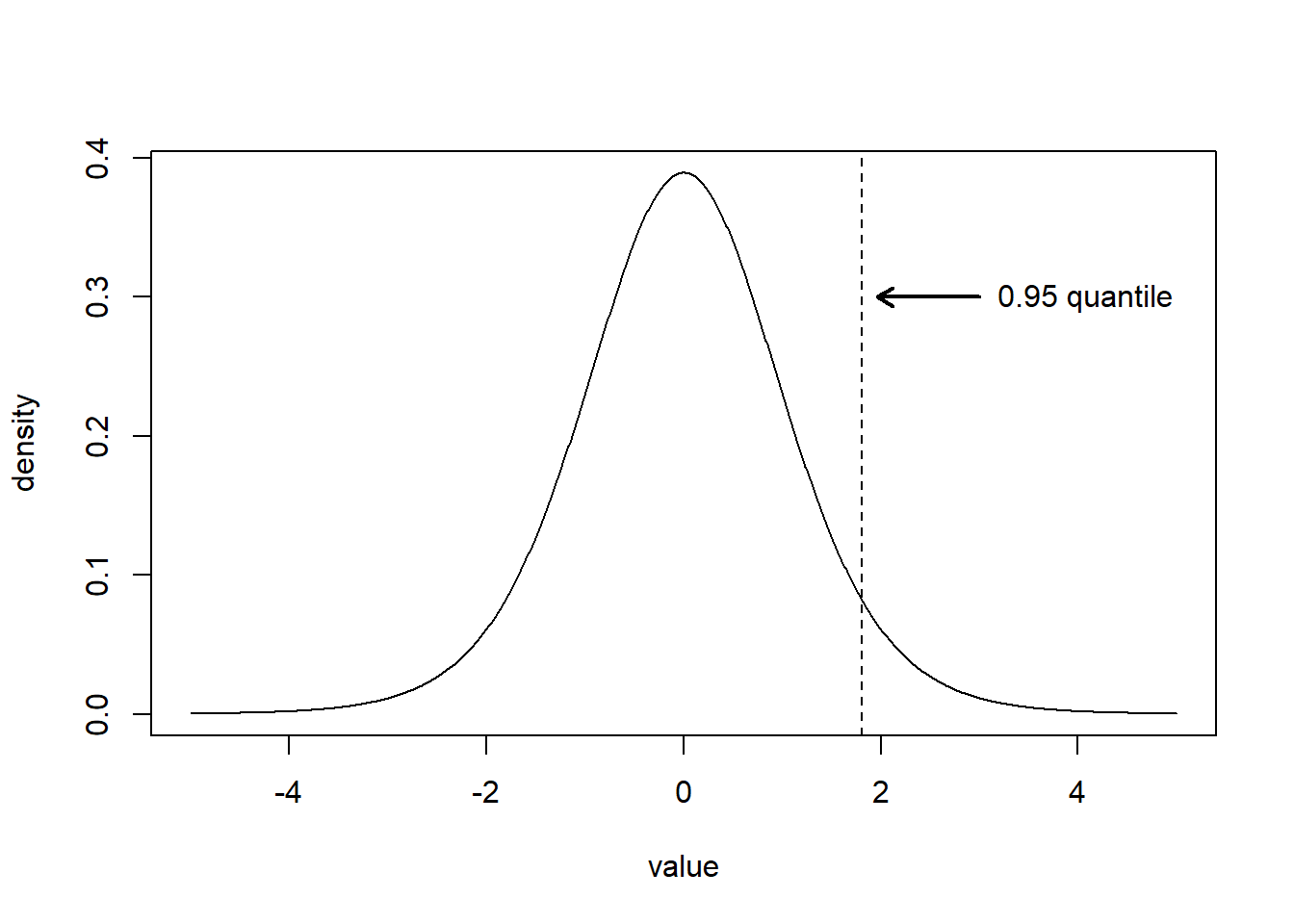
Figure 6.1: The solid line shows the density of a \(t\) random variable with 10 degrees of freedom. The dashed vertical line indicates \(t^{0.05}_{10}\), the 0.95 quantile of a \(t\) distribution with 10 degrees of freedom. The area to the left of the line is 0.95 while the area to the right is 0.05.

We use the notation \(F_{\nu_1, \nu_2}\) to denote a random variable having an \(F\) distribution with \(\nu_1\) numerator degrees of freedom and \(\nu_2\) denominator degrees of freedom. We let \(F^{\alpha}_{\nu_1,\nu_2}\) denote the \(1-\alpha\) quantile of an \(F\) random variables with \(\nu_1\) numerator degrees of freedom and \(\nu_2\) denominator degrees of freedom. In fact, \([t_{\nu}]^2=F_{1,\nu}\), i.e., the square of a \(t\) random variable with \(\nu\) degrees of freedom is equivalent to an \(F\) random variable with \(1\) numerator degree of freedom and \(\nu\) denominator degrees of freedom.

6.3 Assumptions and properties of the OLS estimator

We continue by reviewing some of the properties of \(\hat{\boldsymbol{\beta}}\), the OLS estimator of the regression coefficient vector.

We assume that \[ \mathbf{y} = \mathbf{X}\boldsymbol{\beta}+\boldsymbol{\epsilon}, \tag{6.1} \] using standard matrix notation.

We also assume that the model in Equation (6.1) is correct (i.e., we have correctly specified the true model that generated the data) and that \[ \boldsymbol{\epsilon}\mid \mathbf{X}\sim \mathsf{N}(\mathbf{0}_{n\times 1},\sigma^2 \mathbf{I}_{n\times n}). \tag{6.2} \] This assumption applies to all errors, so we believe that all errors, observed and future, will have mean 0, variance \(\sigma^2\), will be uncorrelated, and have a normal distribution.

Under these assumptions, we showed in Chapter 5 that

\[ \mathbf{y}\mid \mathbf{X}\sim \mathsf{N}(\mathbf{X}\boldsymbol{\beta}, \sigma^2 \mathbf{I}_{n\times n}). \] and \[\hat{\boldsymbol{\beta}}\mid \mathbf{X} \sim \mathsf{N}(\boldsymbol{\beta}, \sigma^2(\mathbf{X}^T\mathbf{X})^{-1}). \tag{6.3} \]

6.4 Parametric confidence intervals for regression coefficients

6.4.1 Standard \(t\)-based confidence intervals

Under the assumptions in Equations (6.1) and (6.2), we can prove (though we won’t) that \[ \frac{\hat{\beta}_j-\beta_j}{\hat{\mathrm{se}}(\hat{\beta}_j)}\sim t_{n-p}, \quad j=0,1,\ldots,p-1, \]

where \(\hat{\mathrm{se}}(\hat{\beta}_j)=\hat{\sigma}\sqrt{(\mathbf{X}^T\mathbf{X})^{-1}_{j+1,j+1}}\) is the estimated standard error of \(\hat{\beta}_j\). Recall that estimated standard error is the estimated standard deviation of the sampling distribution of \(\hat{\beta}_j\). Also, recall that the notation \((\mathbf{X}^T\mathbf{X})^{-1}_{j+1,j+1}\) indicates the element in row \(j+1\), column \(j+1\), of the matrix \((\mathbf{X}^T\mathbf{X})^{-1}\). Thus, \((\hat{\beta}_j-\beta_j)/\hat{\mathrm{se}}(\hat{\beta}_j)\) is a pivotal quantity with a \(t\) distribution, and it can be used to derive a confidence interval

A confidence interval for \(\beta_j\) with confidence level \(1-\alpha\) is given by the expression \[ \hat{\beta}_j \pm t^{\alpha/2}_{n-p} \hat{\mathrm{se}}(\hat{\beta}_j),\quad j=0,2,\ldots,p-1. \tag{6.4} \] It is critical to note that the \(1-\alpha\) confidence level refers to the procedure for a single interval, not the family of intervals we can produce for all \(p\) coefficients. We discuss this issue in more detail in Section 6.5.

The confint function returns confidence intervals for the regression coefficients of a fitted model. Technically, the confint function is a generic function that has methods for many different object classes, but we only discuss its usage with lm objects. The confint function has 3 main arguments:

• object: a fitted model object. In our case, the object produced by the lm function.
• parm: a vector of numbers or names indicating the parameters for which we want to construct confidence intervals. By default, confidence intervals are constructed for all parameters.
• level: the confidence level desired for the confidence interval. The default value is 0.95, which will produce 95% confidence intervals.

We once again use the penguins data from the palmerpenguins package (Horst, Hill, and Gorman 2022) to illustrate what we have learned. Consider the regression model \[ \begin{aligned} &E(\mathtt{bill\_length\_mm}\mid \mathtt{body\_mass\_g}, \mathtt{flipper\_length\_mm}) \\ &=\beta_0+\beta_1 \mathtt{body\_mass\_g} + \beta_2 \mathtt{flipper\_length\_mm}. \end{aligned} \]

We estimate the parameters of this model in R using the code below.

# load data
data(penguins, package = "palmerpenguins")
# fit model
mlmod <- lm(bill_length_mm ~ body_mass_g + flipper_length_mm, data = penguins)

We obtain the 95% confidence intervals for the 3 regression coefficients by running the code below.

confint(mlmod)
##                           2.5 %      97.5 %
## (Intercept)       -1.244658e+01 5.573192182
## body_mass_g       -4.534709e-04 0.001777908
## flipper_length_mm  1.582365e-01 0.285494420

The 95% confidence interval for the intercept parameter is [-12.45, 5.58]. We are 95% confident that the mean penguin bill length is between -12.25 and 5.58 mm for a penguin with a body mass of 0 g and a flipper length of 0 mm. (This really isn’t sensible).

The 95% confidence interval for the body_mass_g coefficient is [-0.00046, 0.002]. We are 95% confident the regression coefficient for body_mass_g is between -0.00046 and 0.002, assuming the flipper_length_mm regressor is also in the model.

If we wanted to get the 90% confidence interval for the flipper_length_mm coefficient by itself, we could use either of the commands shown below.

# two styles for determining the CI for a single parameter (at a 90% level)
confint(mlmod, parm = 3, level = 0.90)
##                         5 %      95 %
## flipper_length_mm 0.1685112 0.2752197
confint(mlmod, parm = "flipper_length_mm", level = 0.90)
##                         5 %      95 %
## flipper_length_mm 0.1685112 0.2752197

We discuss how to “manually” construct these intervals using R in Section 6.11.1.

6.5 The multiple comparisons problem

Our linear models typically have multiple regression coefficients, and thus, we typically want to construct confidence intervals for all of the coefficients.

While individual confidence intervals have utility in providing us with plausible values of the unknown coefficients, the confidence level of the procedure described in Section 6.4.1 is only valid for a single interval. Since we are constructing multiple intervals, the simultaneous confidence level of the procedure for the family of intervals is less than \(1-\alpha\). This is an example of the multiple comparisons problem.

A multiple comparisons problem occurs anytime we make multiple inferences (confidence intervals, hypothesis tests, prediction intervals, etc.). We are more likely to draw erroneous conclusions if we do not adjust for the fact that we are making multiple inferential statements. E.g., a confidence interval procedure with level 0.95 will produce intervals that contain the target parameter with probability 0.95. If we construct two confidence intervals with level 0.95, then the family-wise confidence level (i.e., the probability that both intervals simultaneously contain their respective target parameters) will be less than 0.95. (We can guarantee that our family-wise confidence level will be at least 0.90, but we can’t determine the exact value without more information). In general, the family-wise confidence level is the probability that a confidence interval procedure produces a family of intervals that simultaneously contain their target parameter. The family-wise confidence level is also known as the simultaneous or overall confidence level.

A multiple comparisons procedure is a procedure designed to adjust for multiple inferences. In the context of confidence intervals, a multiple comparisons procedure will produce a family of intervals that have a family-wise confidence level above some threshold. We discuss two basic multiple comparisons procedures for confidence intervals below.

6.5.1 Adjusted confidence intervals for regression coefficients

Bonferroni (1936) proposed a simple multiple comparisons procedure that is applicable in many contexts. This general procedure is known as the Bonferroni correction. We describe its application below.

Suppose we are constructing \(k\) confidence intervals simultaneously. We control the family-wise confidence level of our intervals at \(1-\alpha\) if we construct the individual confidence intervals with the level \(1-\alpha/k\). We sketch a proof of this below.

Boole’s inequality (Boole 1847) states that for a countable set of events \(A_1, A_2, A_3 \ldots\), \[P(\cup_{j=1}^\infty A_j) \leq \sum_{j=1}^\infty P(A_j).\] This is a generalization of the fact that \[ P(A \cup B) = P(A) + P(B) - P(A\cap B) \leq P(A) + P(B) \] for two events \(A\) and \(B\). We can use Boole’s inequality to show that the Bonferroni correction controls the family-wise confidence level of our confidence intervals at \(1-\alpha\).

Suppose that we construct a family of \(k\) confidence intervals with individual confidence level \(1-\alpha/k\) (and all assumptions are satisfied.) Then the probability that the confidence interval procedure for a specific interval doesn’t contain the target parameter is \(\alpha/k\). Then \[ \begin{aligned} & P(\mbox{All }k\mbox{ intervals contain the target parameter}) \\ & = 1 - P(\mbox{At least one of the }k\mbox{ intervals misses the target parameter}) \\ & = 1 - P(\cup_{j=1}^k \mbox{interval }j\mbox{ misses the target parameter}) \\ & \geq 1 - \sum_{j=1}^k P(\mbox{interval }j\mbox{ misses the target parameter}) \\ & = 1 - k(\alpha/k) \\ &= 1-\alpha. \end{aligned} \] Thus, the family-wise confidence level of all \(k\) intervals is AT LEAST \(1-\alpha\) when the Bonferroni correction is used.

The Bonferroni correction is known to be conservative, which means that the family-wise confidence level is typically much larger than \(1-\alpha\). This might sound like a desirable property, but conservative methods can have low power. In the context of our confidence intervals, this means our intervals are much wider than they need to be, so we aren’t able to draw precise conclusions about the plausible values of our regression coefficients.

Let’s construct simultaneous confidence intervals for our penguins example using the Bonferroni correction. If we want to control the family-wise confidence level of our \(k=3\) intervals at \(0.95\), then \(\alpha = 0.05\) and the Bonferroni correction suggests that we should construct the individual intervals at a confidence level of \(1-0.05/3=0.983\). We construct the Bonferroni-adjusted confidence intervals using the code below.

# Simultaneous 95% confidence intervals for mlmod
confint(mlmod, level = 1 - 0.05/3)
##                         0.833 %    99.167 %
## (Intercept)       -1.445714e+01 7.583749811
## body_mass_g       -7.024372e-04 0.002026874
## flipper_length_mm  1.440377e-01 0.299693234

Alternatively, we can use the confint_adjust function from the api2lm package (French 2023) to construct this interval. The confint_adjust function works identically to the confint function except that it has an additional argument to indicate the type of adjustment to make when constructing the confidence intervals. Specifying method = "bonferroni" will produce Bonferroni-corrected intervals, as demonstrated in the code below.

library(api2lm)
confint_adjust(mlmod, method = "bonferroni")
## 
## Bonferroni-adjusted confidence intervals
## 
## Family-wise confidence level of at least 0.95 
## 
##               term           lwr         upr
##        (Intercept) -1.445714e+01 7.583749811
##        body_mass_g -7.024372e-04 0.002026874
##  flipper_length_mm  1.440377e-01 0.299693234

Working and Hotelling (1929) developed another multiple comparisons procedure that can be used to preserve the family-wise confidence level of the intervals at \(1-\alpha\). The Working-Hotelling multiple comparisons procedure is valid for ALL linear combinations of the regression coefficients, meaning that we can construct an arbitrarily large number of confidence intervals for linear combinations of the regression coefficients with this procedure and the family-wise confidence level will be at least \(1-\alpha\) (Weisberg 2014).

The Working-Hotelling procedure guarantees that if we construct the individual confidence intervals in the following way, then the family-wise confidence level will be at least \(1-\alpha\): \[ \hat{\beta}_j \pm \sqrt{p F^\alpha_{p,n-p}} \hat{\mathrm{se}}(\hat{\beta}_j),\quad j=0,2,\ldots,p-1. (\#eq:wh-ci-betas) \]

The confint_adjust function from the api2lm package will produce these intervals when setting the method argument to "wh". We construct Working-Hotelling-adjusted intervals with family-wise confidence level of at least 0.95 for the penguins example using the code below.

# 95% family-wise CIs using Working-Hotelling
confint_adjust(mlmod, method = "wh")
## 
## Working-Hotelling-adjusted confidence intervals
## 
## Family-wise confidence level of at least 0.95 
## 
##               term           lwr         upr
##        (Intercept) -1.630614e+01 9.432751051
##        body_mass_g -9.313981e-04 0.002255835
##  flipper_length_mm  1.309798e-01 0.312751116

In this example, the Bonferroni-adjusted intervals are narrower than the Working-Hotelling-adjusted intervals. The Working-Hotelling intervals tends to be narrower for small \(p\) (e.g., \(p=1\) or \(2\)) and small \(n-p\) (e.g., \(n-p = 1\) or \(2\)) (Mi and Sampson 1993). Additionally, as the number of intervals increases, the Working-Hotelling intervals will eventually be narrower than the Bonferroni-adjusted intervals.

6.6 Prediction: mean response versus new response

It is common to make two types of predictions in a regression context: prediction of a mean response and prediction of a new response. In either context, we want to make predictions with respect to a specific combination of regressor values, which we denote \(\mathbf{x}_0\). Using our previous notation, the mean response for a specific combination of regressors is denoted \(E(Y\mid \mathbb{X}=\mathbf{x}_0)\). We do not have notation to describe a new response for a specific combination of regressor values, so we will use the notation \(Y(\mathbf{x}_0)\).

\(E(Y\mid \mathbb{X}=\mathbf{x}_0)\) represents the average response when the regressor values are \(\mathbf{x}_0\). Conceptually, this is the number we would get if were able to determine the average of an infinite number of responses with regressor values being fixed at \(\mathbf{x}_0\).

\(Y(\mathbf{x}_0)\) represents the actual response we will will observe for a new observation with regressor values \(\mathbf{x}_0\). Conceptually, we can think of \(Y(\mathbf{x}_0)\) as the mean response for that combination of regressor values plus some error, or more formally, \[ Y(\mathbf{x}_0)=E(Y\mid \mathbb{X}=\mathbf{x}_0)+\epsilon(\mathbf{x}_0), \] where \(\epsilon(\mathbf{x_0})\) denotes the error for our new observation.

Suppose we want to rent a new apartment or buy a new house. If we look through the available listings, we will likely filter our search results by certain characteristics. We might limit our search to dwellings with 3 bedrooms, 2 bathrooms, that are within a certain distance of public transportation, and have a certain amount of square footage. If we averaged the monthly rent or asking price of all the dwellings matching our specifications, then that would be an approximation of the mean response for that combination of specifications (i.e., regressors). We would need all the possible dwellings matching those characteristics to get the true average. This average would give us an idea of the “typical” price of dwellings with those characteristics. On the other hand, we likely want to know the price of the dwelling we actually end up in. This is the “new response” we want to predict.

Though we can discuss predictions for both the mean response and a new response, it is common to distinguish the two scenarios by using the terminology “estimating the mean response” to refer to prediction of the the mean and “prediction a new response” when we want to predict a new observation. We use this convention in what follows to distinguish the two contexts.

6.7 Confidence interval for the mean response

Consider a typical linear regression model with \(p\) regression coefficients given by

\[E(Y|\mathbb{X})=\beta_0+\beta_1 X_1 + \ldots \beta_{p-1} X_{p-1}.\]

We want to estimate the mean response for a specific combination of regressor values. The mean response for that combination of regressors is obtained via the equivalent expressions

\[ \begin{aligned} E(Y\mid \mathbb{X}=\mathbf{x}_0) &= \beta_0 + \sum_{j=1}^{p-1}x_{0,j}\beta_j \\ &= \mathbf{x}_0^T \boldsymbol{\beta}. \end{aligned} \]

To simplify our notation, we drop the “\(\mathbb{X}=\)” in our discussion below, so \(E(Y\mid \mathbb{X}=\mathbf{x}_0)\equiv E(Y\mid \mathbf{x}_0)\).

What does \(E(Y\mid \mathbf{x}_0)\) represent? It represents the average response we will observe if we somehow managed to observe infinitely many responses with \(\mathbb{X}=\mathbf{x}_0\).

The Gauss-Markov Theorem discussed in Chapter 3 indicates that the best linear unbiased estimator of the mean response is given by the equation\[ \begin{aligned} \hat{E}(Y\mid \mathbf{x}_0) &= \hat{\beta}_0 + \sum_{j=1}^{p-1}x_{0,j}\hat{\beta}_j \\ &= \mathbf{x}_0^T \hat{\boldsymbol{\beta}}, \end{aligned} \]

which replaces the unknown, true coefficients by their OLS estimates.

We want to create a confidence interval for \(E(Y\mid \mathbf{x}_0)\). If we divide the estimation error of the mean response, i.e., \(E(Y\mid \mathbf{x}_0)-\hat{E}(Y\mid \mathbf{x}_0)\), by its estimated standard deviation, then we obtain a pivotal quantity. More specifically, we have

\[ \frac{E(Y\mid \mathbf{x}_0)-\hat{E}(Y\mid \mathbf{x}_0)}{\sqrt{\hat{\mathrm{var}}\left(E(Y\mid \mathbf{x}_0)-\hat{E}(Y\mid \mathbf{x}_0)\right)}} = \frac{E(Y\mid \mathbf{x}_0)- \mathbf{x}_0^T \hat{\boldsymbol{\beta}}}{ \hat{\mathrm{se}}(\mathbf{x}_0^T\hat{\boldsymbol{\beta}})}\sim t_{n-p}, \]

with

\[ \hat{\mathrm{se}}(\mathbf{x}_0^T\hat{\boldsymbol{\beta}})=\hat{\sigma}\sqrt{\mathbf{x}_0^T (\mathbf{X}^T \mathbf{X})^{-1}\mathbf{x}_0}. \tag{6.5} \]

A confidence interval for \(E(Y\mid \mathbf{x}_0)\) with confidence level \(1-\alpha\) is given by the expression

\[ \mathbf{x}_0^T\hat{\boldsymbol{\beta}} \pm t^{\alpha/2}_{n-p} \hat{\mathrm{se}}(\mathbf{x}_0^T\hat{\boldsymbol{\beta}}). \tag{6.6} \]

The predict function is a generic function used to make predictions based on fitted models. We can use this function to estimate the mean response for multiple combinations of predictor variables, compute the estimated standard error of each estimate, and obtain confidence intervals for the mean response. The primary arguments to the lm method for predict are:

• object: A fitted model from the lm function.
• newdata: A data frame of predictor values. All predictors used in the formula used to fit object must be provided. Each row contains the predictor values for the mean response we want to estimate. If this is not provided, then the fitted values for each observation are returned.
• se.fit: A logical value indicating whether we want to explicitly compute the standard errors of each estimated mean, i.e., \(\hat{\mathrm{se}}(\mathbf{x}_0^T \hat{\boldsymbol{\beta}})\) for each estimate.
• interval: The type of interval to compute. The default is none, meaning no interval is provided. Setting interval = "confidence" will return a confidence interval for the mean response associated with each row of newdata. Setting interval = "prediction" will return a prediction interval for a new response, which we will discuss in the next section.
• level: The confidence level of the interval.

Run ?predict.lm in the Console for additional details about this function.

We will estimate the mean response for the parallel lines model previously fit to the penguins data. We do this to emphasize the fact that the predict function asks you to specify the values of the predictor variables for each estimate you want to make, not the complete set of regressors.

Recall that in Section 3.9, we fit a parallel lines model to the penguins data that used both body_mass_g and species to explain the behavior of bill_length_mm. Letting \(D_C\) denote the indicator variable for the Chinstrap level and \(D_G\) denote the indicator variable for the Gentoo level, the fitted parallel lines model was \[ \begin{aligned} &\hat{E}(\mathtt{bill\_length\_mm} \mid \mathtt{body\_mass\_g}, \mathtt{species})\\ &= 24.92 + 0.004 \mathtt{body\_mass\_g} + 9.92 D_C + 3.56 D_G. \end{aligned} \] We fit this model below, assigning it the name lmodp.

# fit parallel lines model to penguins data
lmodp <- lm(bill_length_mm ~ body_mass_g + species,
            data = penguins)
coef(lmodp)
##      (Intercept)      body_mass_g speciesChinstrap 
##     24.919470977      0.003748497      9.920884113 
##    speciesGentoo 
##      3.557977539

Let’s estimate the mean response for the “typical” body_mass_g of each species. We compute the mean body_mass_g of each species using the code below, assigning the resulting data frame the name newpenguins. We use the group_by and summarize functions from the dplyr package (Wickham, François, et al. 2023) to simplify this process.

# mean body_mass_g of each species
newpenguins <- penguins |>
  dplyr::group_by(species) |>
  dplyr::summarize(body_mass_g = mean(body_mass_g, na.rm = TRUE))
newpenguins
## # A tibble: 3 × 2
##   species   body_mass_g
##   <fct>           <dbl>
## 1 Adelie          3701.
## 2 Chinstrap       3733.
## 3 Gentoo          5076.

We now have a data frame with variables for the two predictors, species and body_mass_g , used to fit lmodp. Each row of newpenguins contains the mean body_mass_g for each level of species and is suitable for use in the predict function.

In the code below, we estimate the mean bill_length_mm based on the fitted model in lmodp for the mean body_mass_g of each level of species. We also choose to compute the estimated standard errors of each estimate by setting the se.fit argument to TRUE.

# estimate mean and standard error for 3 combinations of predictors
predict(lmodp, newdata = newpenguins, se.fit = TRUE)
## $fit
##        1        2        3 
## 38.79139 48.83382 47.50488 
## 
## $se.fit
##         1         2         3 
## 0.1955643 0.2914228 0.2166833 
## 
## $df
## [1] 338
## 
## $residual.scale
## [1] 2.403134

An Adelie penguin with a body mass of 3700.662 g is estimated to have a mean bill length of 38.79 mm with an estimated standard error of 0.196 mm. A Chinstrap penguin with a body mass of 3733.09 g is estimated to have a mean bill length of 48.83 mm with an estimated standard error of 0.29 mm. A Gentoo penguin with a body mass of 5076.02 g is estimated to have a mean bill length of 47.50 mm with an estimated standard error of 0.22 mm.

To compute the 98% confidence intervals for the mean response for each combination of predictors, we specify level = 0.98 and interval = "confidence" in the predict function in the code below.

predict(lmodp, newdata = newpenguins, level = 0.98, interval = "confidence")
##        fit      lwr      upr
## 1 38.79139 38.33427 39.24851
## 2 48.83382 48.15264 49.51500
## 3 47.50488 46.99840 48.01136

The 98% confidence interval for the mean bill length of an Adelie penguin with a body mass of 3700.662 g is [38.33, 39.25] mm. We are 98% confident that the mean bill length of Adelie penguins with a body mass of 3700.662 g is between 38.33 and 39.25 mm. Note: we are constructing a confidence interval for the mean bill length of ALL Adelie penguins with this body mass, i.e., for

\[ E(\mathtt{flipper\_length\_mm}\mid \mathtt{body\_mass\_g} = 3700.662, \mathtt{species} = \mathtt{Adelie}), \]

which is an unknown characteristic of the population of all Adelie penguins. Similarly, the 98% confidence interval for the mean bill length of Chinstrap penguins with a body mass of 3733.09 g is [48.15, 49.52] mm. Lastly, the mean flipper length of Gentoo penguins with a body mass of 5076.02 g is [46.99, 48.02] mm.

We provide details about manually computing confidence intervals for the mean response in Section 6.11.3.

We are once again faced with a multiple comparisons problem because we are making 3 inferences. To control the family-wise confidence level of our intervals, we can use the Bonferroni or Working-Hotelling corrections previously discussed in Section 6.5.1. Both corrections are implemented in the predict_adjust function in the api2lm package, which is intended to work identically to the predict function, but produces intervals that adjust for multiple comparisons. The only additional argument is method, with choices "none" (no correction), "bonferroni" (Bonferroni adjustment), or "wh" (Working-Hotelling adjustment). We produce both types of adjusted intervals in the code below. The Bonferroni-adjusted confidence intervals are slightly narrower in this example.

# bonferroni-adjusted confidence intervals for the mean response
predict_adjust(lmodp, newdata = newpenguins, level = 0.98,
               interval = "confidence", method = "bonferroni")
## 
## Bonferroni-adjusted confidence intervals
## 
## Family-wise confidence level of at least 0.98 
## 
##        fit      lwr      upr
## 1 38.79139 38.25751 39.32527
## 2 48.83382 48.03826 49.62939
## 3 47.50488 46.91335 48.09641
# working-hotelling-adjusted confidence intervals for the mean response
predict_adjust(lmodp, newdata = newpenguins, level = 0.98,
               interval = "confidence", method = "wh")
## 
## Working-Hotelling-adjusted confidence intervals
## 
## Family-wise confidence level of at least 0.98 
## 
##        fit      lwr      upr
## 1 38.79139 38.11858 39.46420
## 2 48.83382 47.83122 49.83642
## 3 47.50488 46.75941 48.25035

6.8 Prediction interval for a new response

We once again assume the regression model \[ E(Y|\mathbb{X})=\beta_0+\beta_1 X_1 + \ldots \beta_{p-1} X_{p-1}. \] We want to predict a new response for a specific combination of regressor values, \(\mathbf{x}_0\). The new response will be the mean response for that combination of regressors, \(E(Y\mid \mathbf{x}_0)\), plus the error for that observation, \(\epsilon(\mathbf{x}_0)\), i.e., \[ Y(\mathbf{x}_0)=E(Y\mid \mathbf{x}_0) + \epsilon(\mathbf{x}_0). \]

Thus, our predicted new response, \(\hat{Y}(\mathbf{x})\) is the estimated mean plus the estimated error, i.e., \[ \hat{Y}(\mathbf{x}_0)=\hat{E}(Y\mid \mathbf{x}_0) + \hat{\epsilon}(\mathbf{x}_0). \] We have already used \(\hat{E}(Y\mid \mathbf{x}_0)=\mathbf{x}_0^T\hat{\boldsymbol{\beta}}\) as the estimator for \(E(Y\mid \mathbf{x}_0)\) since it is the best linear unbiased estimator according to the Gauss-Markov theorem. What should we use for \(\hat{\epsilon}(\mathbf{x}_0)\)? In short, because all of the errors, \(\epsilon_1, \epsilon_2,\ldots, \epsilon_n, \epsilon(\mathbf{x}_0)\) are uncorrelated and have a normal distribution with mean zero, our best guess is the mean value of the errors, which is zero. This is not true when the errors are correlated, but we do not discuss that in detail. Thus, the best predictor of a new response is \[ \begin{aligned} \hat{Y}(\mathbf{x}_0) &=\hat{E}(Y\mid \mathbf{x}_0) + \hat{\epsilon}(\mathbf{x}_0)\\ &= \mathbf{x}_0^T\hat{\boldsymbol{\beta}} + 0 \\ &= \mathbf{x}_0^T\hat{\boldsymbol{\beta}}. \end{aligned} \]

We want to create a prediction interval for \(Y(\mathbf{x}_0)\). A prediction interval is basically the same thing as a confidence interval, but the interval estimator is for a random variable instead of a parameter. If we divide the estimation error of the new response, i.e., \(Y(\mathbf{x}_0)-\hat{Y}(\mathbf{x}_0)\), by its estimated standard deviation, \(\widehat{\mathrm{sd}}(Y(\mathbf{x}_0)-\hat{Y}(\mathbf{x}_0))\), then we obtain a \(t\)-distributed pivotal quantity \[ \frac{Y(\mathbf{x}_0)-\hat{Y}(\mathbf{x}_0)}{\widehat{\mathrm{sd}}(Y(\mathbf{x}_0)-\hat{Y}(\mathbf{x}_0))} \sim t_{n-p}, \] where \[ \widehat{\mathrm{sd}}(Y(\mathbf{x}_0)-\hat{Y}(\mathbf{x}_0))=\hat{\sigma}\sqrt{1 + \mathbf{x}_0^T (\mathbf{X}^T \mathbf{X})^{-1}\mathbf{x}_0}. \tag{6.7} \]

The standard deviation of the prediction error is sometimes known as the standard error of prediction, but we do not use that terminology. A detailed derivation of \(\widehat{\mathrm{sd}}(Y(\mathbf{x}_0)-\hat{Y}(\mathbf{x}_0))\) is provided in Section 6.11.4.

A prediction interval for \(Y(\mathbf{x}_0)\) with confidence level \(1-\alpha\) is given by the expression \[ \mathbf{x}_0\hat{\boldsymbol{\beta}} \pm t^{\alpha/2}_{n-p} \hat{\mathrm{sd}}(Y(\mathbf{x}_0)-\hat{Y}(\mathbf{x}_0)). (\#eq:t-pi-new-response) \]

There is a conceptual and mathematical relationship between the standard deviation of the estimation error for the mean response and the prediction error for a new observation. If we compare the expressions for \(\hat{\mathrm{se}}(\mathbf{x}_0^T\hat{\boldsymbol{\beta}})\) in Equation (6.5) and \(\widehat{\mathrm{sd}}(Y(\mathbf{x}_0)-\hat{Y}(\mathbf{x}_0))\) in Equation (6.7), we see that that \[ \hat{\mathrm{sd}}(Y(\mathbf{x}_0)-\hat{Y}(\mathbf{x}_0)) = \hat{\sigma} + \hat{\mathrm{se}}(\mathbf{x}_0^T\hat{\boldsymbol{\beta}}). \] Because of this, prediction intervals for a new response are always wider than a confidence interval for the mean response when considering the same regressor values, \(\mathbf{x}_0\), and confidence level. Conceptually, prediction intervals are wider because there are two sources of uncertainty in our prediction: estimating the mean response and predicting the error of the new response. Estimating the mean response does not require us to predict the error of a new response, so the uncertainty of our estimate is less. We can see that this is formally true through the derivations provided in Section 6.11.4.

The predict function can be used to create predictions and prediction intervals for a new response in the same way that it can be used to estimate the mean response and produce associated confidence intervals. If the interval argument is "none", then predictions for a new response are returned. As we have already seen, \(\hat{E}(Y\mid \mathbf{x}_0)\) and \(\hat{Y}(\mathbf{x}_0)\) are the same number. If the interval argument is "prediction", then the predicted new response and associated prediction interval will be produced for each row of data supplied to the newdata argument.

Continuing the example started in Section 6.7, we want to predict the response value for new, unobserved penguins having the observed mean body_mass_g for each level of species. The fitted model is stored in lmodp and the data frame with the predictors for the new responses is stored in newpenguins. We print the coefficients of the fitted model and the data frame of new predictors below for clarity.

coef(lmodp)
##      (Intercept)      body_mass_g speciesChinstrap 
##     24.919470977      0.003748497      9.920884113 
##    speciesGentoo 
##      3.557977539
newpenguins
## # A tibble: 3 × 2
##   species   body_mass_g
##   <fct>           <dbl>
## 1 Adelie          3701.
## 2 Chinstrap       3733.
## 3 Gentoo          5076.

In the code below, we predict the bill_length_mm for new penguins for the predictor values stored in newpenguins based on the fitted model in lmodp. We also construct the associated 99% prediction intervals.

# predict new response and compute prediction intervals
# for 3 combinations of predictors
predict(lmodp, newdata = newpenguins,
        interval = "prediction", level = 0.99)
##        fit      lwr      upr
## 1 38.79139 32.54561 45.03718
## 2 48.83382 42.56301 55.10464
## 3 47.50488 41.25442 53.75534

A new Adelie penguin with a body mass of 3700.662 g is predicted to have a bill length of 38.79 mm. We are 99% confident that a new Adelie penguins with a body mass of 3700.662 g will have a flipper length between 32.54 and 45.04 mm. Similarly, the 99% prediction interval for the bill length of a new Chinstrap penguin with a body mass of 3733.09 g is [48.56, 55.11] mm. The flipper length of a new Gentoo penguin with a body mass of 5076.02 g is between 41.25 and 53.75 mm with a confidence level of 0.99.

Since we are making 3 predictions, our inferences suffer from the multiple comparisons problem. To control the family-wise confidence level of our intervals, we can use the Bonferroni correction with \(k=3\). The Working-Hotelling correction discussed in Section 6.5.1 does not apply to new responses. However, a similar adjustment proposed by Scheffé does apply (Kutner et al. 2005). The prediction interval multiplier used for a single prediction interval with confidence level \(1-\alpha\) changes from \(t^{\alpha/2}_{n-p}\) to \(\sqrt{k F^{\alpha}_{k,n-p}}\) to control the family-wise confidence level at \(1-\alpha\) for a family of \(k\) prediction intervals. Recall that the Working-Hotelling multiplier was \(\sqrt{p F^{alpha}_{p,n-p}}\). Thus, the Scheffé multiplier scales with the number of predictions being made while the Working-Hotelling multiplier scales with the number of estimated regression coefficients in the fitted model.

Both the Bonferroni and Scheffé multiple comparisons corrections are implemented in the predict_adjust function in the api2lm package. In the prediction interval setting, we can choose the correction method argument to be "none" (no correction), "bonferroni" (Bonferroni adjustment), or "scheffe" (Scheffé adjustment). We produce both types of adjusted intervals in the code below. The Bonferroni-adjusted confidence intervals are slightly narrower in this example.

# bonferroni-adjusted prediction intervals for new responses
predict_adjust(lmodp, newdata = newpenguins, level = 0.99,
               interval = "prediction",
               method = "bonferroni")
## 
## Bonferroni-adjusted prediction intervals
## 
## Family-wise confidence level of at least 0.99 
## 
##        fit      lwr      upr
## 1 38.79139 31.66373 45.91905
## 2 48.83382 41.67760 55.99004
## 3 47.50488 40.37188 54.63787
# sheffe-adjusted prediction intervals for new responses
predict_adjust(lmodp, newdata = newpenguins, level = 0.99,
               interval = "prediction",
               method = "scheffe")
## 
## Scheffe-adjusted prediction intervals
## 
## Family-wise confidence level of at least 0.99 
## 
##        fit      lwr      upr
## 1 38.79139 30.60787 46.97492
## 2 48.83382 40.61751 57.05014
## 3 47.50488 39.31523 55.69453

6.9 Hypothesis tests for a single regression coefficient

If we assume we are fitting the multiple linear regression model in Equation (6.1), then our model has \(p\) regression coefficient \(\beta_0, \beta_1, \ldots, \beta_{p-1}\). How can we perform a hypothesis test for exactly one of these regression coefficients?

Let’s say we wish to test whether, for this model, \(\beta_j\) differs from some constant number \(c\) (typically, \(c=0\)). Let \(\boldsymbol{\beta}_{-j}=\boldsymbol{\beta}\setminus{\beta_j}\), i.e., \(\boldsymbol{\beta}_{-j}\) is the vector of all regression coefficients except \(\beta_j\). \(\boldsymbol{\beta}_{-j}\) has \(p-1\) elements. We can state the hypotheses we wish to test as \[ \begin{aligned} H_0: \beta_j &= c \mid \boldsymbol{\beta}_{-j}\in\mathbb{R}^{p-1} \\ H_a: \beta_j &\neq c \mid \boldsymbol{\beta}_{-j}\in\mathbb{R}^{p-1}. \end{aligned} \tag{6.8} \] The first part of the null hypothesis in Equation (6.8) states that \(\beta_j = c\) while the first part of the alternative hypothesis assumes that \(\beta_j \neq c\). But what does the second half of the hypotheses mean? The vertical bar means “assuming or conditional on”, similar to the notation you would see in conditional probabilities or distributions. What this means is that we are performing the hypothesis test while assuming that the other coefficients are some real number (possibly even zero). Why state this at all? Isn’t it implicitly assumed? No. We could perform a hypothesis test for \(\beta_j\) for many different models that have differing regressors. By writing out hypotheses in the style of Equation (6.8), we are being very clear that we are performing a test for \(\beta_j\) in the context of the model that has the regressors associated with \(\boldsymbol{\beta}_{-j}\). Tests are model specific, so it is important to be clarify the exact model under consideration

Recall that if we make the assumptions in Equation (6.2), then

\[\begin{equation} \frac{\hat{\beta}_j-\beta_j}{\hat{\mathrm{se}}(\hat{\beta}_j)}\sim t_{n-p}, \quad j=0,1,\ldots,p-1. \tag{6.9} \end{equation}\]

How do the hypotheses in Equation (6.8) affect the pivotal quantity in Equation (6.9)? Under the null hypothesis, the statistic \[ T_j = \frac{\hat{\beta}_j-c}{\hat{\mathrm{se}}(\hat{\beta}_j)} \sim t_{n-p}. \] Thus, the null distribution of \(T_j\) is a \(t\) distribution with \(n-p\) degrees of freedom. We emphasize that this is only true if the assumptions in Equation (6.2) are true.

The p-value associated with this test is computed via the equation \[ p\text{-value} = 2P(t_{n-p}\geq |T_j|). \] What if we wished to test a one-sided hypothesis? The p-value for a lower-tailed test is \(p\text{-value}=P(t_{n-p}\leq T_j)\) while the p-value for an upper-tailed test is \(p\text{-value}=P(t_{n-p}\geq T_j)\).

We will perform a hypothesis test for the model \[ \begin{aligned} &E(\mathtt{bill\_length\_mm}\mid \mathtt{body\_mass\_g}, \mathtt{flipper\_length\_mm}) \\ &=\beta_0+\beta_1 \mathtt{body\_mass\_g} + \beta_2 \mathtt{flipper\_length\_mm} \end{aligned} \]

for the penguins data. The fitted model is assigned the name mlmod. Suppose we want to test

\[ \begin{aligned} H_0: &\beta_1 = 0 \mid \beta_0\in \mathbb{R}, \beta_2 \in \mathbb{R} \\ H_a: &\beta_1 \neq 0 \mid \beta_0\in \mathbb{R}, \beta_2 \in \mathbb{R}. \end{aligned} \] R conveniently provides this information in the output of the summary function (specifically, the coefficients element if we don’t want extra information). We extract this information from the mlmod object in the code below.

summary(mlmod)$coefficients
##                        Estimate   Std. Error    t value
## (Intercept)       -3.4366939266 4.5805531903 -0.7502792
## body_mass_g        0.0006622186 0.0005672075  1.1675067
## flipper_length_mm  0.2218654584 0.0323484492  6.8586119
##                       Pr(>|t|)
## (Intercept)       4.536070e-01
## body_mass_g       2.438263e-01
## flipper_length_mm 3.306943e-11

Moving from left to right, the first column (no name) indicates the coefficient term under consideration, the second column (Estimate) provides the estimated coefficients, the third column (Std. Error) provides the estimated standard error (i.e., \(\hat{\mathrm{se}}(\hat{\beta}_j)\)) for each coefficient, the fourth column (t value) provides the test statistic associated with testing \(H_0: \beta_j = 0 \mid \boldsymbol{\beta}_{-j} \in \mathbb{R}^{p-1}\) versus a suitable alternative for each coefficient, while the final column (Pr(>|t|)) provides the two-tailed p-value associated with this test.

Thus, for our test of the body_mass_g coefficient, the test statistic is \(T_1 = 1.17\) and the associated p-value is 0.24. There is no evidence that the coefficient for body_mass_g differs from zero, assuming the model also allows for the inclusion of the intercept and flipper_length_mm coefficients.

6.10 Hypothesis tests for multiple regression coefficients

Suppose we have a standard linear regression model with \(p\) regression coefficients such as the one defined in Equation (6.1). We refer to this model as the “Complete Model”.

We want to compare the Complete Model to a “Reduced Model”. The Reduced Model is a special case of the Complete Model. Alternatively, we can say the Reduced Model is nested in the Complete Model. We use the abbreviations RM to indicate the Reduced Model and CM to indicate the Complete Model.

The most common examples of Reduced Model are:

1. All of the coefficients except the intercept are set to zero.
2. Some of the coefficients are set to zero.

Other examples of a RM set certain coefficients equal to each other or place other restrictions on the coefficients.

Let \(RSS_{RM}\) denote the RSS of the RM and \(RSS_{CM}\) denote the RSS of the CM. Similarly, \(\mathrm{df}_{RM}\) and \(\mathrm{df}_{CM}\) denote the degrees of freedom associated with the RSS for the RM and CM, respectively. Recall that the degrees of freedom associated with a RSS is simply \(n\), the number of observations used to fit the model, minus the number of estimated regression coefficients in the model being considered.

We want to perform a hypothesis test involving multiple regression coefficients in our model. Without be specific or developing complex notation, we cannot be precise in stating the hypotheses we wish to test. A general statement of the hypotheses we will test are:

\[ \begin{aligned} &H_0: \text{RM is an adequate model for describing the population.} \\ &H_a: \text{CM is a more appropriate model for describing the population.} \end{aligned} \]

We wish to statistically assess whether we can simplify our model from \(CM\) to \(RM\). If \(RM\) doesn’t adequately explain the patterns of the data, then we will conclude that \(CM\) is a more appropriate model.

If we assume that the assumptions in Equation (6.2) are true for \(RM\) and that \(RM\) is the true model, then

\[ F=\frac{\frac{RSS_{RM}-RSS_{CM}}{\mathrm{df}_{RM}-\mathrm{df}_{CM}}}{\frac{RSS_{CM}}{\mathrm{df}_{CM}}}=\frac{\frac{RSS_{RM}-RSS_{CM}}{\mathrm{df}_{RM}-\mathrm{df}_{CM}}}{\hat{\sigma}^2_{CM}}\sim F_{\mathrm{df}_{RM}-\mathrm{df}_{CM},\mathrm{df}_{CM}}, \tag{6.10} \] where \(F_{\mathrm{df}_{RM}-\mathrm{df}_{CM},\mathrm{df}_{CM}}\) is an \(F\) random variable with \(\mathrm{df}_{RM}-\mathrm{df}_{CM}\) numerator degrees of freedom and \(\mathrm{df}_{CM}\) denominator degrees of freedom and \(\hat{\sigma}^2_{CM}\) is the estimated error variance of \(CM\).

The p-value for this test is

\[ p\text{-value}=P(F_{\mathrm{df}_{RM}-\mathrm{df}_{CM},\mathrm{df}_{CM}} \geq F). \]

We consider two common uses for this test below.

6.10.1 Test for a regression relationship

The most common test involving multiple parameters is to test whether any of the non-intercept regression coefficients differ from zero. This test is known as the “test for a regression relationship”.

In this situation, the hypotheses to be tested may be stated as

\[ \begin{aligned} &H_0: E(Y \mid \mathbb{X}) = \beta_0 \\ &H_a: E(Y\mid \mathbb{X}) = \beta_0 + X_1\beta_1 + \cdots + X_{p-1}\beta_{p-1}. \end{aligned} \]

Alternatively, we can state these hypotheses as

\[ \begin{aligned} &H_0: \beta_1 = \cdots = \beta_{p-1} = 0 \mid \beta_0 \in \mathbb{R} \\ &H_a: \beta_1 \in \mathbb{R} \text{ or } \ldots \text{ or } \beta_{p-1}\in \mathbb{R} \mid \beta_0 \in \mathbb{R}. \end{aligned} \]

Notice that the RM in \(H_0\) is a special case of the CM in \(H_a\) with all of the regression coefficients set equal to zero except for the intercept term. Notice that we specifically conditioned our hypotheses on the intercept coefficient, \(\beta_0\), being included in both models we are comparing.

The \(F\) statistic in Equation (6.10) used for this test simplifies dramatically when performing a test for a regression relationship.Using a bit of calculus or by carefully using the OLS estimator of the regression coefficients, it is possible to show that for the Reduced Model that \(\hat{\beta}_0=\bar{Y}\). Thus, for the \(RSS_{RM} = \sum_{i=1}^n (Y_i - \bar{Y})^2\), which is the definition of the TSS defined in Chapter 3! Then the numerator of our F statistic becomes \(TSS - RSS_{CM}\), which is mathematically equivalent to the regression sum of squares for the Complete Model. The degrees of freedom of \(RSS_{RM} = n - 1\). Similarly, the degrees of freedom of \(RSS_{CM} = n - p\). Thus \(\mathrm{df}_{RM} - \mathrm{df}_{CM} = (n - 1) - (n - p) = p-1\). Thus, Our F statistic for this test simplifies to

\[ F = \frac{SS_{reg}/(p-1)}{RSS_{CM}/(n-p)}= \frac{SS_{reg}/(p-1)}{\hat{\sigma}^2_{CM}}, \] where \(SS_{reg}\) is for the CM.

Using the penguins data, let’s perform a test for a regression relationship for the model

\[ \begin{aligned} &E(\mathtt{bill\_length\_mm}\mid \mathtt{body\_mass\_g}, \mathtt{flipper\_length\_mm}) \\ &=\beta_0+\beta_1 \mathtt{body\_mass\_g} + \beta_2 \mathtt{flipper\_length\_mm}. \end{aligned} \]

The fitted model is stored in mlmod.

We are testing

\[ \begin{aligned} &H_0: E(\mathtt{bill\_length\_mm}\mid \mathtt{body\_mass\_g}, \mathtt{flipper\_length\_mm}) = \beta_0 \\ &H_a: E(\mathtt{bill\_length\_mm} \mid \mathtt{body\_mass\_g}, \mathtt{flipper\_length\_mm}) = \beta_0 + \beta_1 \mathtt{body\_mass\_g} + \beta_{2} \mathtt{flipper\_length\_mm}. \end{aligned} \] This can also be stated as

\[ \begin{aligned} &H_0: \beta_1 = \beta_2 = 0 \mid \beta_0 \in \mathbb{R} \\ &H_a: \beta_1 \neq 0 \text{ or } \beta_2 \neq 0 \mid \beta_0 \in \mathbb{R}. \end{aligned} \]

We can get the necessary information for the test for a regression relationship by using the summary function on mlmod.

summary(mlmod)
## 
## Call:
## lm(formula = bill_length_mm ~ body_mass_g + flipper_length_mm, 
##     data = penguins)
## 
## Residuals:
##     Min      1Q  Median      3Q     Max 
## -8.8064 -2.5898 -0.7053  1.9911 18.8288 
## 
## Coefficients:
##                     Estimate Std. Error t value Pr(>|t|)
## (Intercept)       -3.4366939  4.5805532  -0.750    0.454
## body_mass_g        0.0006622  0.0005672   1.168    0.244
## flipper_length_mm  0.2218655  0.0323484   6.859 3.31e-11
##                      
## (Intercept)          
## body_mass_g          
## flipper_length_mm ***
## ---
## Signif. codes:  
## 0 '***' 0.001 '**' 0.01 '*' 0.05 '.' 0.1 ' ' 1
## 
## Residual standard error: 4.124 on 339 degrees of freedom
##   (2 observations deleted due to missingness)
## Multiple R-squared:  0.4329, Adjusted R-squared:  0.4295 
## F-statistic: 129.4 on 2 and 339 DF,  p-value: < 2.2e-16

The necessary information is in the last line of the summary output.

F-statistic: 129.4 on 2 and 339 DF,  p-value: < 2.2e-16

The test statistic for this test is 129.4 with a p-value close to 0.

There is very strong evidence that at least one of the regression coefficients for body_mass_g or flipper_length_mm is non-zero in the regression model for bill_length_mm that already includes an intercept.

Alternatively, the model regressing bill_length_mm on the intercept, body_mass_g, and flipper_length_mm is preferred to the model that has only an intercept.

6.10.2 A more general F test

Let us consider a more general F test where multiple regression coefficients are set to zero. In general, the associated test statistic won’t simplify in any standard way.

We will illustrate the more general F test using the penguins data.

Suppose we want to decide between the simple linear regression model and the parallel lines model for the penguins data.

We want to test between

\[ \begin{aligned} &H_0: E(\mathtt{bill\_length\_mm} \mid \mathtt{body\_mass\_g}, \mathtt{species})\\ &\qquad= \beta_{0} + \beta_1 \mathtt{body\_mass\_g} \\ &H_a: E(\mathtt{bill\_length\_mm} \mid \mathtt{body\_mass\_g}, \mathtt{species})\\ &\qquad = \beta_{0} + \beta_1 \mathtt{body\_mass\_g} + \beta_2 D_C + \beta_3 D_G, \end{aligned} \] where \(D_C\) and \(D_G\) denote the indicator variables for the Chinstrap and Gentoo level of penguin species.

Alternatively, we could state this as

\[ \begin{aligned} &H_0: \beta_2 = \beta_3 = 0 \mid \beta_0 \in \mathbb{R}, \beta_1 \in \mathbb{R}\\ &H_a: \beta_2 \neq 0 \text{ or } \beta_3 \neq 0 \mid \beta_0\in \mathbb{R}, \beta_1 \in \mathbb{R}. \end{aligned} \]

To perform our test, we must fit both models. We fit the simple linear regression model in the code below.

lmod <- lm(bill_length_mm ~ body_mass_g, data = penguins)
coef(lmod)
##  (Intercept)  body_mass_g 
## 26.898872424  0.004051417

We then fit the parallel lines model.

lmodp <- lm(bill_length_mm ~ body_mass_g + species, data = penguins)
coef(lmodp)
##      (Intercept)      body_mass_g speciesChinstrap 
##     24.919470977      0.003748497      9.920884113 
##    speciesGentoo 
##      3.557977539

We use the anova function to get the test statistic and p-value for our general F test. We supply the fitted \(RM\) as the first argument to the function and then the fitted \(CM\) as the second argument. We do that in the code below.

anova(lmod, lmodp)
## Analysis of Variance Table
## 
## Model 1: bill_length_mm ~ body_mass_g
## Model 2: bill_length_mm ~ body_mass_g + species
##   Res.Df    RSS Df Sum of Sq      F    Pr(>F)    
## 1    340 6564.5                                  
## 2    338 1952.0  2    4612.5 399.35 < 2.2e-16 ***
## ---
## Signif. codes:  
## 0 '***' 0.001 '**' 0.01 '*' 0.05 '.' 0.1 ' ' 1

The test statistic (F) is 399.35 and the associated p-value (Pr(>F)) is close to 0.

The is very strong evidence that the parallel lines model is preferred to the simple linear regression model for the penguins data.

We can do another test that compares the parallel lines model to the separate lines model for the penguins data.

We want to choose between

\[ \begin{aligned} &H_0: E(\mathtt{bill\_length\_mm} \mid \mathtt{body\_mass\_g}, \mathtt{species}) \\ &=\qquad \beta_{0} + \beta_1 \mathtt{body\_mass\_g} + \beta_2 D_C + \beta_3 D_G \\ &H_a: E(\mathtt{bill\_length\_mm} \mid \mathtt{body\_mass\_g}, \mathtt{species}) \\ &\qquad = \beta_{0} + \beta_1 \mathtt{body\_mass\_g} + \beta_2 D_C + \beta_3 D_G + \beta_4 \mathtt{body\_mass\_g} D_C + \beta_5 \mathtt{body\_mass\_g} D_G. \end{aligned} \]

Alternatively, we could state this as

\[ \begin{aligned} &H_0: \beta_4 = \beta_5 = 0 \mid \{\beta_0, \beta_1, \beta_2, \beta_3\} \in \mathbb{R}^4.\\ &H_a: \beta_4 \neq 0 \text{ or } \beta_5 \neq 0 \mid \{\beta_0, \beta_1, \beta_2, \beta_3\} \in \mathbb{R}^4. \end{aligned} \]

We now fit the separate lines regression model to the penguins data.

lmods <- lm(bill_length_mm ~ body_mass_g + species + body_mass_g:species,
            data = penguins)
coef(lmods)
##                  (Intercept)                  body_mass_g 
##                26.9941391367                 0.0031878758 
##             speciesChinstrap                speciesGentoo 
##                 5.1800537287                -0.2545906615 
## body_mass_g:speciesChinstrap    body_mass_g:speciesGentoo 
##                 0.0012748183                 0.0009029956

We once again use the anova function to get our associated test statistic and p-value, as shown in the code below.

anova(lmodp, lmods)
## Analysis of Variance Table
## 
## Model 1: bill_length_mm ~ body_mass_g + species
## Model 2: bill_length_mm ~ body_mass_g + species + body_mass_g:species
##   Res.Df    RSS Df Sum of Sq      F Pr(>F)
## 1    338 1952.0                           
## 2    336 1933.4  2    18.596 1.6159 0.2003

The test statistic for this test is 1.62 with an associated p-value of 0.20. It appears that for the model regressing bill_length_mm on body_mass_g and species, the parallel lines model is adequate and we do not need the additional complexity of the separate lines model.

6.11 Going deeper

6.11.1 Manual calculation of the standard \(t\)-based confidence interval for a regression coefficient

Consider the summary of the fitted linear model below, which summarizes a first-order linear model fit to the penguins data earlier in this chapter.

summary(mlmod)
## 
## Call:
## lm(formula = bill_length_mm ~ body_mass_g + flipper_length_mm, 
##     data = penguins)
## 
## Residuals:
##     Min      1Q  Median      3Q     Max 
## -8.8064 -2.5898 -0.7053  1.9911 18.8288 
## 
## Coefficients:
##                     Estimate Std. Error t value Pr(>|t|)
## (Intercept)       -3.4366939  4.5805532  -0.750    0.454
## body_mass_g        0.0006622  0.0005672   1.168    0.244
## flipper_length_mm  0.2218655  0.0323484   6.859 3.31e-11
##                      
## (Intercept)          
## body_mass_g          
## flipper_length_mm ***
## ---
## Signif. codes:  
## 0 '***' 0.001 '**' 0.01 '*' 0.05 '.' 0.1 ' ' 1
## 
## Residual standard error: 4.124 on 339 degrees of freedom
##   (2 observations deleted due to missingness)
## Multiple R-squared:  0.4329, Adjusted R-squared:  0.4295 
## F-statistic: 129.4 on 2 and 339 DF,  p-value: < 2.2e-16

If we want to manually produce 95% confidence intervals for the true regression coefficients for this model using Equation (6.4), then we need to acquire some basic information. We need:

• the estimated regression coefficients
• the degrees of freedom for the fitted model \(n-p\)
• the \(1-\alpha/2\) quantile of a \(t\) random variable with \(n-p\) degrees of freedom
• the estimated standard error of the estimated regression coefficients.

The estimated regression coefficients can be extracted from our fitted model, mlmod, using the coef function. We extract and print the estimated coefficients using the code below while simultaneously assigning the vector the name betahats.

# extract estimated coefficients from mlmod
(betahats <- coef(mlmod))
##       (Intercept)       body_mass_g flipper_length_mm 
##     -3.4366939266      0.0006622186      0.2218654584

The degrees of freedom \(n-p\) is referred to as the residual degrees of freedom and can be obtained by using the df.residual function on the fitted model. Using the code below, we see that the residual degrees of freedom is 339 (this information was also in the summary of the fitted model).

df.residual(mlmod)
## [1] 339

To construct a 95% confidence interval for our coefficients, we need to determine the \(0.975\) quantile of a \(t\) random variable with 339 degrees of freedom. This can be found using the qt function, as is done in the code below. We assign this value the name mult. Notice that value is a bit above 1.96, which is the value often seen in introductory statistics courses for confidence intervals based on the standard normal distribution (\(\mathsf{N}(0,1)\) distribution).

(mult <- qt(0.975, df = 339))
## [1] 1.966986

The estimated standard errors of each coefficient are shown in the summary of the fitted model. They are (approximately) 4.58, 0.00057, and 0.032 and can be obtained by extracting the 2nd column of the coefficients element produced by the summary function.

(sehats <- summary(mlmod)$coefficients[,2])
##       (Intercept)       body_mass_g flipper_length_mm 
##      4.5805531903      0.0005672075      0.0323484492

A alternative approach is to use 3 step process below:

1. Use the vcov function to obtain the estimated variance matrix of \(\hat{\boldsymbol{\beta}}\), i.e., \(\hat{\mathrm{var}}(\hat{\boldsymbol{\beta}})\).
2. Use the diag function to extract the diagonal elements of this matrix, which gives us \(\hat{\mathrm{var}}(\hat{\beta}_0), \hat{\mathrm{var}}(\hat{\beta}_1), \ldots, \hat{\mathrm{var}}(\hat{\beta}_{p-1})\).
3. Use the sqrt function to calculate the estimated standard errors from the estimated variances of the estimated coefficients.

We use this process in the code below, which returns the same estimated standard errors we previously obtained.

# 2nd approach to obtaining estimated standard errors
sqrt(diag(vcov(mlmod)))
##       (Intercept)       body_mass_g flipper_length_mm 
##      4.5805531903      0.0005672075      0.0323484492

Using the estimated coefficients (betahats), the appropriate quantile of the \(t\) distribution (mult), and the estimated standard errors (sehats), we can manually produce the standard t-based confidence intervals using the code below.

data.frame(lb = betahats - mult * sehats,
           ub = betahats + mult * sehats)
##                              lb          ub
## (Intercept)       -1.244658e+01 5.573192182
## body_mass_g       -4.534709e-04 0.001777908
## flipper_length_mm  1.582365e-01 0.285494420

6.11.2 Details about estimation of the mean response

Consider the estimated mean response for a specific combination of regressor values, denoted by \(\mathbf{x}_0\), so that \[\hat{E}(Y\mid \mathbf{x}_0)=\mathbf{x}_0^T\hat{\boldsymbol{\beta}}.\]

Using some of the matrix-related results from Appendix B and the result in Equation (6.3), we can determine that \[ \begin{aligned} \mathrm{var}\left(\hat{E}(Y \mid \mathbf{x}_0)\right) &= \mathrm{var}(\mathbf{x}_0^T \hat{\boldsymbol{\beta}}) \\ &= \mathbf{x}_0^T \mathrm{var}(\hat{\boldsymbol{\beta}})\mathbf{x}_0\\ &= \sigma^2 \mathbf{x}_0^T (\mathbf{X}^T \mathbf{X})^{-1}\mathbf{x}_0. \end{aligned} \tag{6.11} \] To get the simplest expression for the confidence interval for \(E(Y\mid\mathbf{x}_0)\), we have to make a number of connections that are often glossed over. We discuss them explicitly. Since the error variance, \(\sigma^2\), in Equation (6.11) isn’t known, we replace it with the typical estimator \(\hat{\sigma}^2=RSS/(n-p)\) to get \[ \hat{\mathrm{var}}\left(\hat{E}(Y\mid\mathbf{x}_0)\right)=\hat{\sigma}^2 \mathbf{x}_0^T (\mathbf{X}^T \mathbf{X})^{-1}\mathbf{x}_0. \tag{6.12} \]

The standard error of an estimator is the standard deviation of the estimator’s variance, so we have \(\mathrm{se}\left(\hat{E}(Y\mid\mathbf{x}_0)\right)=\sqrt{\mathrm{var}\left(\hat{E}(Y\mid \mathbf{x}_0)\right)}\). Similarly, we have that the estimated standard error for \(\hat{E}(Y\mid \mathbf{x}_0)\) is \(\hat{\mathrm{se}}\left(\hat{E}(Y\mid\mathbf{x}_0)\right)=\sqrt{\hat{\mathrm{var}}\left(\hat{E}(Y\mid \mathbf{x}_0)\right)}\). Taking the square root of Equation (6.12), we see that \[ \hat{\mathrm{se}}\left(\hat{E}(Y\mid \mathbf{x}_0)\right)=\hat{\sigma} \sqrt{\mathbf{x}_0^T (\mathbf{X}^T \mathbf{X})^{-1}\mathbf{x}_0}. \]

Additionally, since \(E(Y\mid \mathbf{x}_0)\) is an (unknown) constant, we also have that \[\mathrm{var}\left(E(Y\mid \mathbf{x}_0)-\hat{E}(Y\mid \mathbf{x}_0)\right)=\mathrm{var}\left(\hat{E}(Y\mid \mathbf{x}_0)\right). \] If we divide the estimation error of the mean response, i.e., \(E(Y\mid \mathbf{x}_0)-\hat{E}(Y\mid \mathbf{x}_0)\), by its estimated standard deviation, then we obtain a pivotal quantity. More specifically, we have \[ \frac{E(Y\mid \mathbf{x}_0)-\hat{E}(Y\mid \mathbf{x}_0)}{\sqrt{\hat{\mathrm{var}}\left(E(Y\mid \mathbf{x}_0)-\hat{E}(Y\mid \mathbf{x}_0)\right)}} = \frac{E(Y\mid \mathbf{x}_0)- \mathbf{x}_0 \hat{\boldsymbol{\beta}}}{ \hat{\mathrm{se}}(\mathbf{x}_0\hat{\boldsymbol{\beta}})}\sim t_{n-p}. \]

6.11.3 Manual calculation of confidence intervals for the mean response

We discuss manual computation of the estimated mean response and associated confidence interval for a particular combination of regressor values based on the penguins example discussed in Section 6.7.

Specifically, we estimate the mean response for the fitted parallel lines model given by\[ \begin{aligned} &\hat{E}(\mathtt{bill\_length\_mm} \mid \mathtt{body\_mass\_g}, \mathtt{species})\\ &= 24.92 + 0.004 \mathtt{body\_mass\_g} + 9.92 D_C + 3.56 D_G, \end{aligned} \] where \(D_C\) and \(D_G\) denote the indicator variables for the Chinstrap and Gentoo levels of the species variable. This fitted model is stored in lmodp. The estimated coefficients are shown in the code below.

coef(lmodp)
##      (Intercept)      body_mass_g speciesChinstrap 
##     24.919470977      0.003748497      9.920884113 
##    speciesGentoo 
##      3.557977539

We want to estimate the mean response for the following combination of predictors stored in the newpenguins data frame, which is printed in the code below.

# mean body_mass_g of each species
newpenguins
## # A tibble: 3 × 2
##   species   body_mass_g
##   <fct>           <dbl>
## 1 Adelie          3701.
## 2 Chinstrap       3733.
## 3 Gentoo          5076.

We want to use the newpenguins data frame to generate the matrix of regressors used to estimate the associated mean responses. We can create the matrix of regressors using the model.matrix function. The main arguments of model.matrix are:

• object: an object of the appropriate class. In our case, it is a formula or fitted model.
• data: a data frame with the predictors needed to construct the matrix.

We need only the right side of the formula used to fit the model in lmodp to create our matrix of regressor values. We can use the formula function to extract the formula used to fit lmodp. We then use model.matrix to create the matrix of regressor by values needed for estimating the mean. The matrix produced by model.matrix, X0, includes a column for the intercept term and the indicator variables in lmodp.

# determine formula used to fit lmodp
formula(lmodp)
## bill_length_mm ~ body_mass_g + species
# create matrix of regressor values from newpenguins
(X0 <- model.matrix(~ body_mass_g + species, data = newpenguins))
##   (Intercept) body_mass_g speciesChinstrap speciesGentoo
## 1           1    3700.662                0             0
## 2           1    3733.088                1             0
## 3           1    5076.016                0             1
## attr(,"assign")
## [1] 0 1 2 2
## attr(,"contrasts")
## attr(,"contrasts")$species
## [1] "contr.treatment"

We can obtain the estimated mean by taking the product of X0 and the estimated coefficients for lmodp. We assign the estimated mean responses the name est_means.

(est_means <- X0 %*% coef(lmodp))
##       [,1]
## 1 38.79139
## 2 48.83382
## 3 47.50488

We now use Equation (6.5) to get the estimated standard error of each estimated mean response. First, we use model.matrix to extract the original matrix of regressors, \(\mathbf{X}\), from the fitted model lmodp. The sigma function is used to extract \(\hat{\sigma}\) from lmodp. Each row of X0 contains a particular instance regressor values. In the code below, we extract each row of X0, and then use Equation (6.5) to compute the estimated standard error associated with each estimated mean response; these are assigned the names se1, se2, and se3. That approach isn’t scalable, so we provide a scalable version of these computations that is assigned the name sehat.

# original matrix of regressors
X <- model.matrix(lmodp)
sigmahat <- sigma(lmodp)
# compute estimated standard error for each estimated mean response
# crossprod(X) = t(X) %*% X
(sehat1 <- sigmahat * sqrt(t(X0[1,]) %*% solve(crossprod(X), X0[1,])))
##           [,1]
## [1,] 0.1955643
(sehat2 <- sigmahat * sqrt(t(X0[2,]) %*% solve(crossprod(X), X0[2,])))
##           [,1]
## [1,] 0.2914228
(sehat3 <- sigmahat * sqrt(t(X0[3,]) %*% solve(crossprod(X), X0[3,])))
##           [,1]
## [1,] 0.2166833
# scalable computation of estimated standard errors
(sehat <- sigmahat * sqrt(diag(X0 %*% solve(crossprod(X), t(X0)))))
##         1         2         3 
## 0.1955643 0.2914228 0.2166833

To finish the computation of our confidence intervals, we determine the correct multiplier, \(t_{n-p}^{\alpha/2}\). For a 98% confidence interval, \(\alpha = 0.02\) and \(\alpha/2 = 0.01\). The degrees of freedom, \(n-p\), is 338 (as shown in the code below). So the multiplier can be represented as \(t_{338}^{0.01}\), which is the \(0.99\) quantile of a \(t\) distribution with 338 degrees of freedom. We provide this information to the qt function, which provides the quantiles of a \(t\) distribution, using the code below to get the correct multiplier.

# degrees of freedom, n-p
df.residual(lmodp)
## [1] 338
# multiplier for confidence interval
(mult <- qt(0.99, df = df.residual(lmodp)))
## [1] 2.337431

Thus, our 98% confidence intervals for each mean response can be computed using the code below, which matches the results we obtained in Section 6.7.

data.frame(lb = est_means - mult * sehat,
           ub = est_means + mult * sehat)
##         lb       ub
## 1 38.33427 39.24851
## 2 48.15264 49.51500
## 3 46.99840 48.01136

6.11.4 Details about prediction interval for a new response

We want to predict the value of a new response for a specific combination of regressor values, \(\mathbf{x}_0\). The value of the new response is denoted by \(Y(\mathbf{x}_0)\) and its prediction by \(\hat{Y}(\mathbf{x}_0)\).

In Section 6.8, we briefly discussed that the new response may be written as \[ Y(\mathbf{x}_0) = E(Y \mid \mathbf{x}_0) + \epsilon(\mathbf{x}_0), \] and that the predicted new response, under our standard assumptions, is given by \[ \hat{Y}(\mathbf{x}_0)=\mathbf{x}_0^T\hat{\boldsymbol{\beta}}. \]

Using these relationships, we can determine that the variance of the prediction error for a new response is given by \[ \begin{aligned} \mathrm{var}\left(Y(\mathbf{x}_0)-\hat{Y}(\mathbf{x}_0)\right) &= \mathrm{var}(Y(\mathbf{x}_0)-\mathbf{x}_0^T \hat{\boldsymbol{\beta}}) \\ &= \mathrm{var}(\mathbf{x}_0^T\boldsymbol{\beta} + \epsilon(\mathbf{x}_0)-\mathbf{x}_0^T \hat{\boldsymbol{\beta}}) \\ \end{aligned} \tag{6.13} \]

Recall from Appendix B that the variance of a constant plus a random variable is equal to the variance of the random variable (since a constant doesn’t vary!). Thus, Equation (6.13) simplifies to \[ \mathrm{var}\left(Y(\mathbf{x}_0)-\hat{Y}(\mathbf{x}_0)\right) = \mathrm{var}(\epsilon(\mathbf{x}_0)-\mathbf{x}_0^T \hat{\boldsymbol{\beta}}). \tag{6.14} \] Using results from Appendix B related to the variance of a sum of random variables, we have that \[ \begin{aligned} &\mathrm{var}\left(Y(\mathbf{x}_0)-\hat{Y}(\mathbf{x}_0)\right) \\ &= \mathrm{var}(\epsilon(\mathbf{x}_0)-\mathbf{x}_0^T \hat{\boldsymbol{\beta}}) \\ &= \mathrm{var}\left(\epsilon(\mathbf{x}_0)\right)+\mathrm{var}(-\mathbf{x}_0^T \hat{\boldsymbol{\beta}}) + 2\mathrm{cov}\left(\epsilon(\mathbf{x}_0), -\mathbf{x}_0^T \hat{\boldsymbol{\beta}}\right) \\ &= \mathrm{var}\left(\epsilon(\mathbf{x}_0)\right)+(-1)^2\mathrm{var}(\mathbf{x}_0^T \hat{\boldsymbol{\beta}}) - 2\mathrm{cov}\left(\epsilon(\mathbf{x}_0), \mathbf{x}_0^T \hat{\boldsymbol{\beta}}\right) \\ &= \mathrm{var}\left(\epsilon(\mathbf{x}_0)\right)+\mathrm{var}(\mathbf{x}_0^T \hat{\boldsymbol{\beta}}) - 2\mathrm{cov}\left(\epsilon(\mathbf{x}_0), \mathbf{x}_0^T \hat{\boldsymbol{\beta}}\right). \end{aligned} \tag{6.15} \]

The covariance term in the final line of Equation (6.15) is 0 because \(\epsilon(\mathbf{x}_0)\) and \(\mathbf{x}_0^T\hat{\boldsymbol{\beta}}\) are uncorrelated. Why are they uncorrelated? Recall that \(\epsilon(\mathbf{x}_0), \epsilon_1, \ldots, \epsilon_n\) are uncorrelated. Also, recall that \(\hat{\boldsymbol{\beta}}=(\mathbf{X}^T\mathbf{X})^{-1}\mathbf{X}^T\mathbf{y}\). Since \(\mathbf{y}=[Y_1,Y_2,\ldots,Y_n]\) and \(Y_i=\mathbf{x}_i^T\boldsymbol{\beta} + \epsilon_i\) for \(i=1,2,\ldots,n\), the “randomness” of \(\mathbf{x}_0^T\hat{\boldsymbol{\beta}}\) comes from \(\epsilon_1, \epsilon_2, \ldots, \epsilon_n\). Since \(\epsilon(\mathbf{x}_0)\) is uncorrelated with \(\epsilon_1, \epsilon_2, \ldots, \epsilon_n\), we conclude that \(\epsilon(\mathbf{x}_0)\) and \(\mathbf{x}_0^T\hat{\boldsymbol{\beta}}\) are uncorrelated, so their covariance is zero. Thus, we have

\[ \begin{aligned} \mathrm{var}\left(Y(\mathbf{x}_0)-\hat{Y}(\mathbf{x}_0)\right) =\mathrm{var}\left(\epsilon(\mathbf{x}_0)\right)+\mathrm{var}(\mathbf{x}_0^T \hat{\boldsymbol{\beta}}) . \end{aligned} \tag{6.16} \] From our assumptions in Section 6.3, we have that \(\mathrm{var}(\epsilon(\mathbf{x}_0))=\sigma^2\). We determined in Section 6.11.2 that \[ \mathrm{var}(\mathbf{x}_0^T\hat{\boldsymbol{\beta}})=\sigma^2 \mathbf{x}_0^T (\mathbf{X}^T \mathbf{X})^{-1}\mathbf{x}_0. \] Using these two facts, we can conclude that \[ \begin{aligned} \mathrm{var}\left(Y(\mathbf{x}_0)-\hat{Y}(\mathbf{x}_0)\right) &=\sigma^2 + \sigma^2 \mathbf{x}_0^T (\mathbf{X}^T \mathbf{X})^{-1}\mathbf{x}_0\\ &=\sigma^2\left(1 + \mathbf{x}_0^T (\mathbf{X}^T \mathbf{X})^{-1}\mathbf{x}_0\right).\\ \end{aligned} \tag{6.17} \] Replacing \(\sigma^2\) by the typical estimator \(\hat{\sigma}^2=RSS/(n-p)\) to get the estimated variance of the prediction error and taking the square root of the estimated variance to get the estimated standard deviation of the prediction error, we have that \[ \widehat{\mathrm{sd}}\left(Y(\mathbf{x}_0)-\hat{Y}(\mathbf{x}_0)\right) = \hat{\sigma}\sqrt{1 + \mathbf{x}_0^T (\mathbf{X}^T \mathbf{X})^{-1}\mathbf{x}_0}. \]