Chapter 3 Linear model estimation

3.1 A simple motivating example

Suppose we observe data related to the heights of 5 mothers and their adult daughters. The observed heights (measured in inches) are provided in Table 3.1. Figure 3.1 displays a scatter plot of the height data provided in Table 3.1. Would it be reasonable to use a mother’s height to predict the height of her adult daughter?

Table 3.1: Heights of mothers and their adult daughters (in).

observation	mother’s height (in)	daughter’s height (in)
1	57.5	61.5
2	60.5	63.5
3	63.5	63.5
4	66.5	66.5
5	69.5	66.5

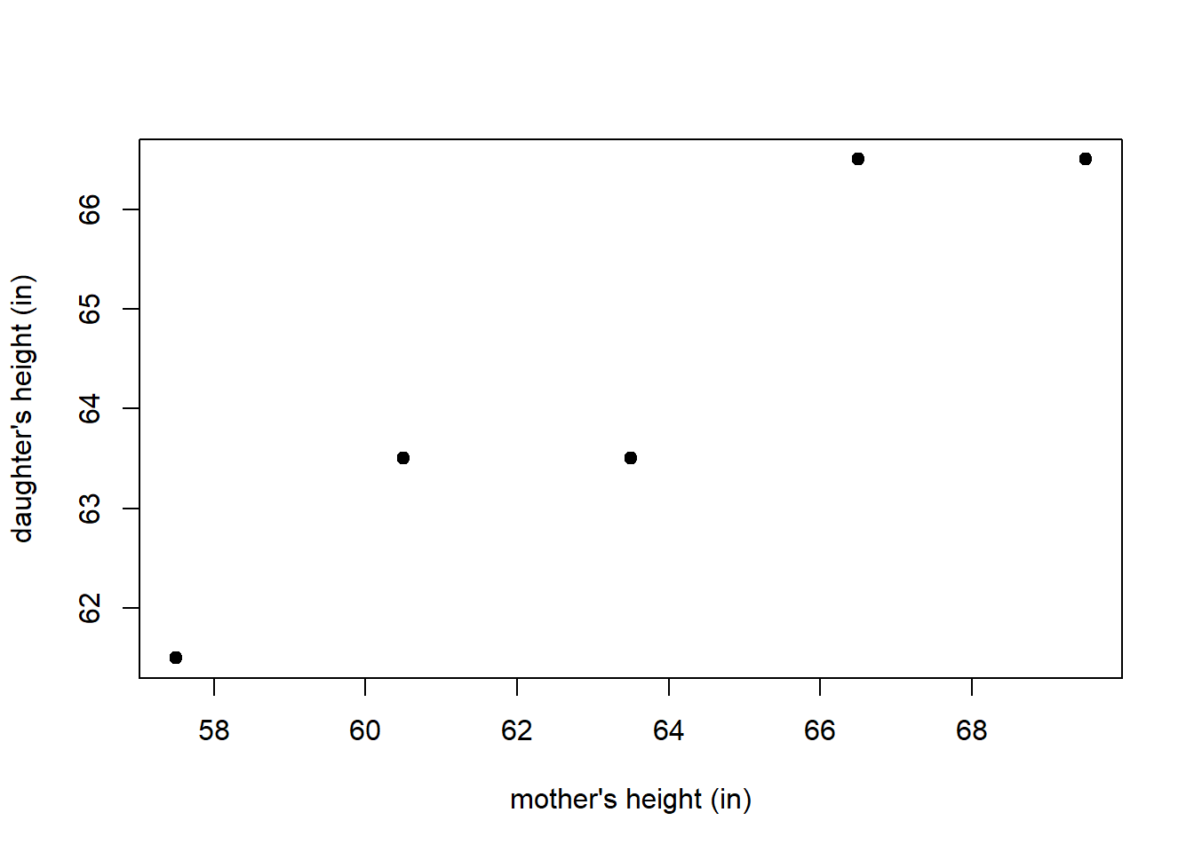
Figure 3.1: A scatter plot displaying pairs of heights for a mother and her adult daughter.

A regression analysis is the process of building a model describing the typical relationship between a set of observed variables. A regression analysis builds the model using observed values of the variables for \(n\) subjects sampled from a population. In the present context, we want to model the height of adult daughters using the height of their mothers. The model we build is known as a regression model.

The variables in a regression analysis may be divided into two types: the response variable and the predictor variables.

The outcome variable we are trying to predict is known as the response variable. Response variables are also known as outcome, output, or dependent variables. The response variable is denoted by \(Y\). The observed value of \(Y\) for observation \(i\) is denoted \(Y_i\).

The variables available to model the response variable are known as predictors variables. Predictor variables are also known as explanatory, regressor, input, independent variables, or simply as features. Following the convention of Weisberg (2014), we use the term regressor to refer to the variables used in our regression model, whether that is the original predictor variable, some transformation of a predictor, some combination of predictors, etc. Thus, every predictor can be a regressor but not all regressors are a predictor. The regressor variables are denoted as \(X_1, X_2, \ldots, X_{p-1}\). The value of \(X_j\) for observation \(i\) is denoted by \(x_{i,j}\). If there is only a single regressor in the model, we can denote the single regressor as \(X\) and the observed values of \(X\) as \(x_1, x_2, \ldots, x_n\).

For the height data, the 5 pairs of observed data are denoted \[(x_1, Y_1), (x_2, Y_2), \ldots, (x_5, Y_5),\] with \((x_i, Y_i)\) denoting the data for observation \(i\). \(x_i\) denotes the mother’s height for observation \(i\) and \(Y_i\) denotes the daughter’s height for observation \(i\). Referring to Table 3.1, we see that, e.g., \(x_3 = 63.5\) and \(Y_5= 66.5\).

Suppose we want to find the straight line that best fits the plot of mother and daughter heights in Figure 3.1. How do we determine the “best fitting” model? Consider Figure 3.2, in which 2 potential “best fitting” lines are drawn on the scatter plot of the height data. Which one is best?

The rest of this chapter focuses on defining and estimating the parameters of a linear regression model. We will start with the simplest type of linear regression, called simple linear regression, which only uses a single regressor variable to model the response. We will then start looking at more complicated linear regression models. After that, we discuss how to evaluate how well an estimated regression model fits the data. We conclude with a summary of some important concepts from the chapter.

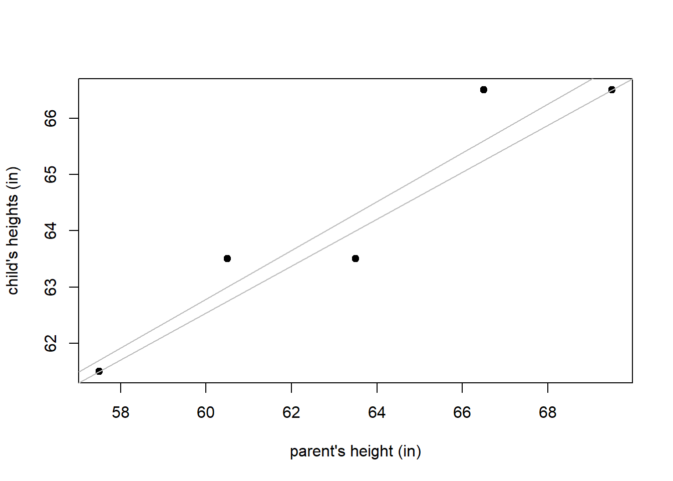
Figure 3.2: Comparison of two potential fitted models to some observed data. The fitted models are shown in grey.

3.2 Estimation of the simple linear regression model

Parameter estimation is the process of using observed data to estimate parameters of a model. There are many different methods of parameter estimation in statistics: method-of-moments, maximum likelihood, Bayesian, etc. The most common parameter estimation method for linear models is the least squares method, which is commonly called Ordinary Least Squares (OLS) estimation. OLS estimation estimates the regression coefficients with the values that minimize the residual sum of squares (RSS), which we will define shortly.

3.2.1 Model definition, fitted values, residuals, and RSS

The regression model for \(Y\) as a function of \(X\), denoted \(E(Y \mid X)\), is the expected value of \(Y\) conditional on the regressor \(X\). Thus, a regression model specifically refers to the expected relationship between the response and regressors.

The simple linear regression model for a response variable assumes the mean of \(Y\) conditional on a single regressor \(X\) is \[ E(Y\mid X) = \beta_0 + \beta_1 X. \]

The response variable \(Y\) is modeled as \[ \begin{aligned} Y &= E(Y \mid X) + \epsilon \\ &= \beta_0 + \beta_1 X + \epsilon, \end{aligned} \tag{3.1} \] where \(\epsilon\) is known as the model error.

The error term \(\epsilon\) is literally the deviation of the response variable from its mean. It is standard to assume that conditional on the regressor variable, the error term has mean 0 and variance \(\sigma^2\), which can be written as \[ E(\epsilon \mid X) = 0 \tag{3.2} \] and \[ \mathrm{var}(\epsilon \mid X) = \sigma^2.\tag{3.3} \]

Using the response values \(Y_1, \ldots, Y_n\) and their associated regressor values \(x_1, \ldots, x_n\), the observed data are modeled as \[ \begin{aligned} Y_i &= \beta_0 + \beta_1 x_i + \epsilon_i \\ &= E(Y\mid X = x_i) + \epsilon_i, \end{aligned} \] for \(i=1\), \(2\),\(\ldots\),\(n\), where \(\epsilon_i\) denotes the error for observation \(i\).

The estimated regression model is defined as \[\hat{E}(Y|X) = \hat{\beta}_0 + \hat{\beta}_1 X,\] where \(\hat{\beta}_j\) denotes the estimated value of \(\beta_j\) for \(j=0,1\).

The \(i\)th fitted value is defined as \[ \hat{Y}_i = \hat{E}(Y|X = x_i) = \hat{\beta}_0 + \hat{\beta}_1 x_i. \tag{3.4} \] Thus, the \(i\)th fitted value is the estimated mean of \(Y\) when the regressor \(X=x_i\). More specifically, the \(i\)th fitted value is the estimated mean response based on the regressor value observed for the \(i\)th observation.

The \(i\)th residual is defined as \[ \hat{\epsilon}_i = Y_i - \hat{Y}_i. \tag{3.5} \] The \(i\)th residual is the difference between the response and estimated mean response of observation \(i\).

The residual sum of squares (RSS) of a regression model is the sum of its squared residuals. The RSS for a simple linear regression model, as a function of the estimated regression coefficients \(\hat{\beta}_0\) and \(\hat{\beta}_1\), is defined as \[ RSS(\hat{\beta}_0, \hat{\beta}_1) = \sum_{i=1}^n \hat{\epsilon}_i^2. \tag{3.6} \]

Using the various objects defined above, there are many equivalent expressions for the RSS. Notably, Equation (3.6) can be rewritten using Equations (3.4) and (3.5) as \[ \begin{aligned} RSS(\hat{\beta}_0, \hat{\beta}_1) &= \sum_{i=1}^n \hat{\epsilon}_i^2 \\ &= \sum_{i=1}^n (Y_i - \hat{Y}_i)^2 & \\ &= \sum_{i=1}^n (Y_i - \hat{E}(Y|X=x_i))^2 \\ &= \sum_{i=1}^n (Y_i - (\hat{\beta}_0 + \hat{\beta}_1 x_i))^2. \end{aligned} \tag{3.7} \]

The fitted model is the estimated model that minimizes the RSS and is written as \[ \hat{Y}=\hat{E}(Y|X) = \hat{\beta}_0 + \hat{\beta}_1 X. \tag{3.8} \] Both \(\hat{Y}\) and \(\hat{E}(Y|X)\) are used to denote a fitted model. \(\hat{Y}\) is used for brevity while \(\hat{E}(Y|X)\) is used for clarity. In a simple linear regression context, the fitted model is known as the line of best fit.

In Figure 3.3, we visualize the response values, fitted values, residuals, and fitted model in a simple linear regression context. Note that:

• The fitted model is shown as the dashed grey line and minimizes the RSS.
• The response values, shown as black dots, are the observed values of \(Y\).
• The fitted values, shown as blue x’s, are the values returned by evaluating the fitted model at the observed regressor values.
• The residuals, shown as solid orange lines, indicate the distance and direction between the observed responses and their corresponding fitted value. If the response is larger than the fitted value then the residual is positive, otherwise it is negative.
• The RSS is the sum of the squared vertical distances between the response and fitted values.

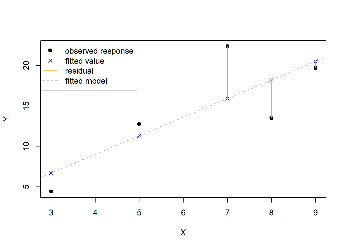
Figure 3.3: Visualization of the fitted model, response values, fitted values, and residuals.

3.2.2 OLS estimators of the simple linear regression parameters

The estimators of \(\beta_0\) and \(\beta_1\) that minimize the RSS for a simple linear regression model can be obtained analytically using basic calculus under minimal assumptions. Specifically, the optimal analytical solutions for \(\hat{\beta}_0\) and \(\hat{\beta}_1\) are valid as long as the regressor values are not a constant value, i.e, \(x_i \neq x_j\) for at least some \(i,j\in \{1,2,\ldots,n\}\).

Define \(\bar{x}=\frac{1}{n}\sum_{i=1}^n x_i\) and \(\bar{Y} = \frac{1}{n}\sum_{i=1}^n Y_i\). The expression \(\bar{x}\) is read “x bar”, and it is the sample mean of the observed \(x_i\) values. The OLS estimators of the simple linear regression coefficients that minimize the RSS are \[ \begin{aligned} \hat{\beta}_1 &= \frac{\sum_{i=1}^n x_i Y_i - \frac{1}{n} \biggl(\sum_{i=1}^n x_i\biggr)\biggl(\sum_{i=1}^n Y_i\biggr)}{\sum_{i=1}^n x_i^2 - \frac{1}{n} \biggl(\sum_{i=1}^n x_i\biggr)^2} \\ &= \frac{\sum_{i=1}^n (x_i - \bar{x})(Y_i - \bar{Y})}{\sum_{i=1}^n (x_i - \bar{x})^2} \\ &= \frac{\sum_{i=1}^n (x_i - \bar{x})Y_i}{\sum_{i=1}^n (x_i - \bar{x})x_i} \end{aligned} \tag{3.9} \] and \[ \hat{\beta}_0 = \bar{Y} - \hat{\beta}_1 \bar{x}. \tag{3.10} \] The various expressions given in Equation (3.9) are equivalent. In fact, in Equation (3.9), all of the numerators are equivalent, and all of the denominators are equivalent. We provide derivations of the estimators for \(\hat{\beta}_0\) and \(\hat{\beta}_1\) in Section 3.12.2.

In addition to the regression coefficients, the other parameter we mentioned in Section 3.2.1 is the error variance, \(\sigma^2\). The most common estimator of the error variance is \[ \hat{\sigma}^2 = \frac{RSS}{\mathrm{df}_{RSS}}. \tag{3.11} \] where \(\mathrm{df}_{RSS}\) is the degrees of freedom of the RSS. In a simple linear regression context, the denominator of Equation (3.11) is \(n-2\). See Section 3.12.1 for more comments about degrees of freedom.

3.3 Penguins simple linear regression example

We will use the penguins data set in the palmerpenguins package (Horst, Hill, and Gorman 2022) to illustrate a very basic simple linear regression analysis.

The penguins data set provides data related to various penguin species measured in the Palmer Archipelago (Antarctica), originally provided by Gorman, Williams, and Fraser (2014). We start by loading the data into memory.

data(penguins, package = "palmerpenguins")

The data set includes 344 observations of 8 variables. The variables are:

• species: a factor indicating the penguin species.
• island: a factor indicating the island the penguin was observed.
• bill_length_mm: a numeric variable indicating the bill length in millimeters.
• bill_depth_mm: a numeric variable indicating the bill depth in millimeters.
• flipper_length_mm: an integer variable indicating the flipper length in millimeters
• body_mass_g: an integer variable indicating the body mass in grams.
• sex: a factor indicating the penguin sex (female, male).
• year: an integer denoting the study year the penguin was observed (2007, 2008, or 2009).

We begin by creating a scatter plot of bill_length_mm versus body_mass_g (y-axis versus x-axis) in Figure 3.4.

plot(bill_length_mm ~ body_mass_g, data = penguins,
     ylab = "bill length (mm)", xlab = "body mass (g)",
     main = "Penguin size measurements")

Figure 3.4: A scatter plot of penguin bill length (mm) versus body mass (g)

We see a clear positive association between body mass and bill length: as the body mass increases, the bill length tends to increase. The pattern is linear, i.e., roughly a straight line.

We will build a simple linear regression model that regresses bill_length_mm on body_mass_g. More specifically, we want to estimate the parameters of the regression model \(E(Y\mid X)=\beta_0+\beta_1\,X\), with \(Y=\mathtt{bill\_length\_mm}\) and \(X=\mathtt{body\_mass\_g}\), i.e., we want to estimate the parameters of the model \[ E(\mathtt{bill\_length\_mm}\mid \mathtt{body\_mass\_g})=\beta_0+\beta_1\,\mathtt{body\_mass\_g}. \]

The lm function uses OLS estimation to fit a linear model to data. The function has two main arguments:

• data: the data frame in which the model variables are stored. This can be omitted if the variables are already stored in memory.
• formula: a Wilkinson and Rogers (1973) style formula describing the linear regression model. For complete details, run ?stats::formula in the Console. If y is the response variable and x is an available numeric predictor, then formula = y ~ x tells lm to fit the simple linear regression model \(E(Y|X)=\beta_0+\beta_1 X\).

We use the code below to fit a linear model regressing bill_length_mm on body_mass_g using the penguins data frame and assign the result the name lmod. lmod is an object of class lm.

lmod <- lm(bill_length_mm ~ body_mass_g, data = penguins) # fit model
class(lmod) # class of lmod
## [1] "lm"

The summary function is commonly used to summarize the results of our fitted model. When an lm object is supplied to the summary function, it returns:

• Call: the function call used to fit the model.
• Residuals: A 5-number summary of the \(\hat{\epsilon}_1, \ldots, \hat{\epsilon}_n\).
• Coefficients: A table that lists:
  • The regressors in the fitted model.
  • Estimate: the estimated coefficient for each regressor.
  • Std. Error: the estimated standard error of the estimated coefficients.
  • t value: the computed test statistic associated with testing \(H_0: \beta_j = 0\) versus \(H_a: \beta_j \neq 0\) for each regression coefficient in the model.
  • Pr(>|t|): the associated p-value of each test.
• Various summary statistics:
  • Residual standard error is the value of \(\hat{\sigma}\), the estimate of the error standard deviation. The degrees of freedom is \(\mathrm{df}_{RSS}\), the number of observations minus the number of estimated coefficients in the model.
  • Multiple R-squared is an estimate of model fit discussed in Section 3.10.
  • Adjusted R-squared is a modified version of Multiple R-squared.
  • F-statistic is the test statistic for the test that compares the model with an only an intercept to the fitted model. The DF (degrees of freedom) values relate to the statistic under the null hypothesis, and the p-value is the p-value for the test.

We use the summary function on lmod to produce the output below.

# summarize results stored in lmod
summary(lmod)
## 
## Call:
## lm(formula = bill_length_mm ~ body_mass_g, data = penguins)
## 
## Residuals:
##      Min       1Q   Median       3Q      Max 
## -10.1251  -3.0434  -0.8089   2.0711  16.1109 
## 
## Coefficients:
##              Estimate Std. Error t value Pr(>|t|)    
## (Intercept) 2.690e+01  1.269e+00   21.19   <2e-16 ***
## body_mass_g 4.051e-03  2.967e-04   13.65   <2e-16 ***
## ---
## Signif. codes:  
## 0 '***' 0.001 '**' 0.01 '*' 0.05 '.' 0.1 ' ' 1
## 
## Residual standard error: 4.394 on 340 degrees of freedom
##   (2 observations deleted due to missingness)
## Multiple R-squared:  0.3542, Adjusted R-squared:  0.3523 
## F-statistic: 186.4 on 1 and 340 DF,  p-value: < 2.2e-16

Using the output above, we see that the estimated parameters are \(\hat{\beta}_0=26.9\) and \(\hat{\beta}_1=0.004\). Thus, our fitted model is \[ \widehat{\mathtt{bill\_length\_mm}}=26.9+0.004 \,\mathtt{body\_mass\_g}. \]

In the context of a simple linear regression model, the intercept term is the expected response when the value of the regressor is zero, while the slope is the expected change in the response when the regressor increases by 1 unit. Thus, based on the model we fit to the penguins data, we can make the following interpretations:

• \(\hat{\beta}_1\): If a penguin has a body mass 1 gram larger than another penguin, we expect the larger penguin’s bill length to be 0.004 millimeters longer.
• \(\hat{\beta}_0\): A penguin with a body mass of 0 grams is expected to have a bill length of 26.9 millimeters.

The latter interpretation is nonsensical. It doesn’t make sense to discuss a penguin with a body mass of 0 grams unless we are talking about an embryo, in which case it doesn’t even make sense to discuss bill length. This is caused by the fact that we are extrapolating far outside the observed body mass values. Our data only includes information for adult penguins, so we should be cautious about drawing conclusions for penguins at other life stages.

The abline function can be used to automatically overlay the fitted model on the observed data. We run the code below to produce Figure 3.5. The fit of the model to our observed data seems reasonable.

plot(bill_length_mm ~ body_mass_g, data = penguins, main = "Penguin size measurements",
     ylab = "bill length (mm)", xlab = "body mass (g)")
# draw fitted line of plot
abline(lmod)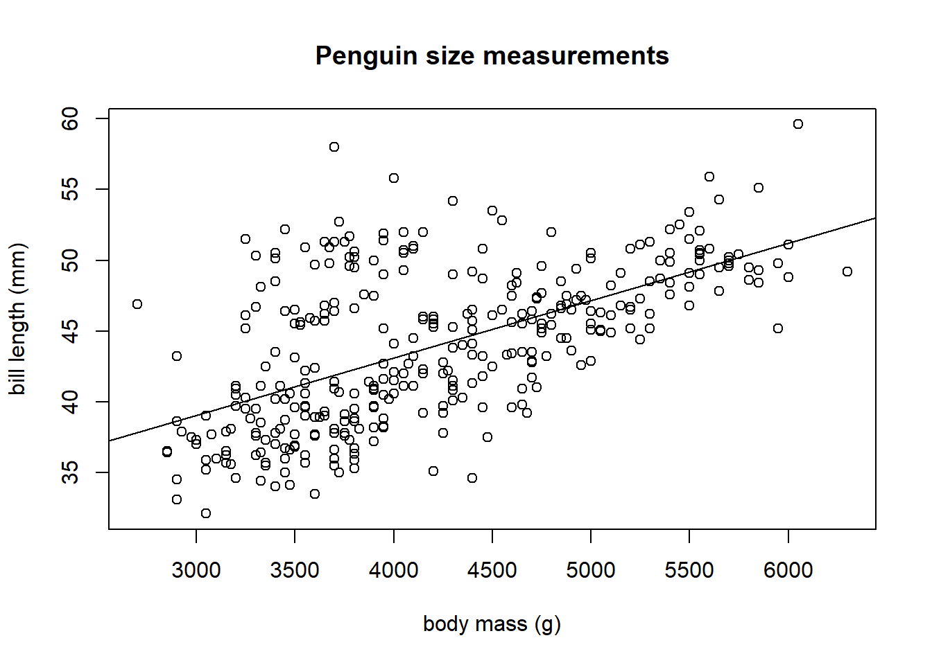

Figure 3.5: The fitted model overlaid on the penguin data.

R provides many additional methods (generic functions that do something specific when applied to a certain type of object) for lm objects. Commonly used ones include:

• residuals: extracts the residuals, \(\hat{\epsilon}_1, \ldots, \hat{\epsilon}_n\) from an lm object.
• fitted: extracts the fitted values, \(\hat{Y}_1, \ldots, \hat{Y}_n\) from an lm object.
• predict: by default, computes \(\hat{Y}_1, \ldots, \hat{Y}_n\) for an lm object. It can also be used to make arbitrary predictions for the lm object.
• coef or coefficients: extracts the estimated coefficients from an lm object.
• deviance: extracts the RSS from an lm object.
• df.residual: extracts \(\mathrm{df}_{RSS}\), the degrees of freedom for the RSS, from an lm object.
• sigma: extracts \(\hat{\sigma}\) from an lm object.

We now use some of the methods to extract important characteristics of our fitted model.

We extract the estimated regression coefficients, \(\hat{\beta}_0\) and \(\hat{\beta}_1\), using the coef function.

(coeffs <- coef(lmod)) # extract, assign, and print coefficients
##  (Intercept)  body_mass_g 
## 26.898872424  0.004051417

We extract the vector of residuals, \(\hat{\epsilon}_1,\ldots, \hat{\epsilon}_n\), using the residuals function.

ehat <- residuals(lmod) # extract and assign residuals
head(ehat) # first few residuals
##          1          2          3          5          6 
## -2.9916846 -2.7942554  0.2340237 -4.1762596 -2.3865430 
##          7 
## -2.6852575

We extract the vector of fitted values, \(\hat{Y}_1,\ldots, \hat{Y}_n\), using the fitted function.

yhat <- fitted(lmod) # extract and assign fitted values
head(yhat) # first few fitted values
##        1        2        3        5        6        7 
## 42.09168 42.29426 40.06598 40.87626 41.68654 41.58526

We can also extract the vector of fitted values using the predict function.

yhat2 <- predict(lmod) # compute and assign fitted values
head(yhat2) # first few fitted values
##        1        2        3        5        6        7 
## 42.09168 42.29426 40.06598 40.87626 41.68654 41.58526

We extract the RSS of the model using the deviance function.

(rss <- deviance(lmod)) # extract, assign, and print rss
## [1] 6564.494

We extract the residual degrees of freedom using the df.residual function.

(dfr <- df.residual(lmod)) # extract n - p
## [1] 340

We extract the estimated error standard deviation, \(\hat{\sigma}=\sqrt{\hat{\sigma}^2}\), using the sigma function. In the code below, we square \(\hat{\sigma}\) to estimate the error variance, \(\hat{\sigma}^2\).

(sigmasqhat <- sigma(lmod)^2) # estimated error variance
## [1] 19.30734

From the output above, we that the the first 3 residuals are -2.99, -2.79, and 0.23. The first 3 fitted values are 42.09, 42.29, and 40.07. The RSS for the fitted model is 6564.49 with 340 degrees of freedom. The estimated error variance, \(\hat{\sigma}^2\), is 19.31.

We use the methods function to obtain a full list of methods available for lm objects using the code below.

methods(class = "lm")
##  [1] add1           alias          anova         
##  [4] case.names     coerce         confint       
##  [7] cooks.distance deviance       dfbeta        
## [10] dfbetas        drop1          dummy.coef    
## [13] effects        extractAIC     family        
## [16] formula        fortify        hatvalues     
## [19] influence      initialize     kappa         
## [22] labels         logLik         model.frame   
## [25] model.matrix   nobs           plot          
## [28] predict        print          proj          
## [31] qr             residuals      rstandard     
## [34] rstudent       show           simulate      
## [37] slotsFromS3    summary        variable.names
## [40] vcov          
## see '?methods' for accessing help and source code

3.4 Defining a linear model

3.4.1 Necessary components and notation

We now wish to discuss linear models in a broader context. We begin by defining notation for the components of a linear model and provide some of their important properties. We repeat some of the previous discussion for clarity.

• \(Y\) denotes the response variable.
  • The response variable is treated as a random variable.
  • We will observe realizations of this random variable for each observation in our data set.
• \(X\) denotes a single regressor variable. \(X_1, X_2, \ldots, X_{p-1}\) denote distinct regressor variables if we are performing regression with multiple regressor variables.
  • The regressor variables are treated as non-random variables.
  • The observed values of the regressor variables are treated as fixed, known values.
• \(\mathbb{X}=\{X_0, X_1,\ldots,X_{p-1}\}\) denotes the collection of all regressors under consideration, though this notation is really only needed in the context of multiple regression. \(X_0\) is usually the constant regressor 1, which is needed to include an intercept in the regression model.
• \(\beta_0\), \(\beta_1\), \(\ldots\), \(\beta_{p-1}\) denote regression coefficients.
  • Regression coefficients are statistical parameters that we will estimate from our data.
  • The regression coefficients are treated as fixed, non-random but unknown values.
  • Regression coefficients are not observable.
• \(\epsilon\) denotes model error.
  • The model error is more accurately described as random variation of each observation from the regression model.
  • The error is treated as a random variable.
  • The error is assumed to have mean 0 for all values of the regressors. We write this as \(E(\epsilon \mid \mathbb{X}) = 0\), which is read as, “The expected value of \(\epsilon\) conditional on knowing all the regressor values equals 0”. The notation “\(\mid \mathbb{X}\)” extends the notation used in Equation (4.3) to multiple regressors.
  • The variance of the errors is assumed to be a constant value for all values of the regressors. We write this assumption as \(\mathrm{var}(\epsilon \mid \mathbb{X})=\sigma^2\).
  • The error is never observable (except in the context of a simulation study where the experimenter literally defines the true model).

3.4.2 Standard definition of linear model

In general, a linear regression model can have an arbitrary number of regressors. A multiple linear regression model has two or more regressors.

A linear model for \(Y\) is defined by the equation \[ \begin{aligned} Y &= \beta_0 + \beta_1 X_1 + \beta_2 X_2 + \cdots + \beta_{p-1} X_{p-1} + \epsilon \\ &= E(Y \mid \mathbb{X}) + \epsilon. \end{aligned} \tag{3.12} \]

We write the linear model in this way to emphasize the fact the response value equals the expected response for that combination of regressor values plus some error. It should be clear from comparing Equation (3.12) with the previous line that \[ E(Y \mid \mathbb{X}) = \beta_0 + \beta_1 X_1 + \beta_2 X_2 + \cdots + \beta_{p-1} X_{p-1}, \] which we prove in Chapter 5.

More generally, one can say that a regression model is linear if the mean function can be written as a linear combination of the regression coefficients and known values created from our regressor variables, i.e., \[ E(Y \mid \mathbb{X}) = \sum_{j=0}^{p-1} c_j \beta_j, \tag{3.13} \] where \(c_0, c_1, \ldots, c_{p-1}\) are known functions of the regressor variables, e.g., \(c_1 = X_1 X_2 X_3\), \(c_3 = X_2^2\), \(c_8 = \ln(X_1)/X_2^2\), etc. Thus, if \(g_0,\ldots,g_{p-1}\) are functions of \(\mathbb{X}\), then we can say that the regression model is linear if it can be written as \[ E(Y\mid \mathbb{X}) = \sum_{j=0}^{p-1} g_j(\mathbb{X})\beta_j. \]

A model is linear because of its form, not the shape it produces. Many of the linear model examples given below do not result in a straight line or surface, but are curved. Some examples of linear regression models are:

• \(E(Y|X) = \beta_0\).
• \(E(Y|X) = \beta_0 + \beta_1 X + \beta_2 X^2\).
• \(E(Y|X_1, X_2) = \beta_0 + \beta_1 X_1 + \beta_2 X_2\).
• \(E(Y|X_1, X_2) = \beta_0 + \beta_1 X_1 + \beta_2 X_2 + \beta_3 X_1 X_2\).
• \(E(Y|X_1, X_2) = \beta_0 + \beta_1 \ln(X_1) + \beta_2 X_2^{-1}\).
• \(E(\ln(Y)|X_1, X_2) = \beta_0 + \beta_1 X_1 + \beta_2 X_2\).
• \(E(Y^{-1}|X_1, X_2) = \beta_0 + \beta_1 X_1 + \beta_2 X_2\).

Some examples of non-linear regression models are:

• \(E(Y|X) = \beta_0 + e^{\beta_1 X}\).
• \(E(Y|X) = \beta_0 + \beta_1 X/(\beta_2 + X)\).

The latter regression models are non-linear models because there is no way to express them using the expression in Equation (3.13).

3.5 Estimation of the multiple linear regression model

Suppose we want to estimate the parameters of a linear model with 1 or more regressors, i.e., when we use the model \[ Y=\beta_0 + \beta_1 X_1 + \cdots + \beta_{p-1} X_{p-1} + \epsilon. \]

The system of equations relating the responses, the regressors, and the errors for all \(n\) observations can be written as \[ Y_i = \beta_0 + \beta_1 x_{i,1} + \beta_2 x_{i,2} + \cdots + \beta_{p-1} x_{i,p-1} + \epsilon_i,\quad i=1,2,\ldots,n. \tag{3.14} \]

3.5.1 Using matrix notation to represent a linear model

We can simplify the linear model described in Equation (3.14) using matrix notation. It may be useful to refer to Appendix A for a brief overview of matrix-related information.

We use the following notation:

• \(\mathbf{y} = [Y_1, Y_2, \ldots, Y_n]\) denotes the column vector containing the \(n\) observed response values.
• \(\mathbf{X}\) denotes the matrix containing a column of 1s and the observed regressor values for \(X_1, X_2, \ldots, X_{p-1}\). This may be written as \[\mathbf{X} = \begin{bmatrix} 1 & x_{1,1} & x_{1,2} & \cdots & x_{1,p-1} \\ 1 & x_{2,1} & x_{2,2} & \cdots & x_{2,p-1} \\ \vdots & \vdots & \vdots & \vdots & \vdots \\ 1 & x_{n,1} & x_{n,2} & \cdots & x_{n,p-1} \end{bmatrix}.\]
• \(\boldsymbol{\beta} = [\beta_0, \beta_1, \ldots, \beta_{p-1}]\) denotes the column vector containing the \(p\) regression coefficients.
• \(\boldsymbol{\epsilon} = [\epsilon_1, \epsilon_2, \ldots, \epsilon_n]\) denotes the column vector contained the \(n\) errors.

The system of equations defining the linear model in Equation (3.14) can be written as \[ \mathbf{y} = \mathbf{X}\boldsymbol{\beta} + \boldsymbol{\epsilon}. \] Thus, matrix notation can be used to represent a system of linear equations. A model that cannot be represented as a system of linear equations using matrices is not a linear model.

3.5.2 Residuals, fitted values, and RSS for multiple linear regression

We now discuss of residuals, fitted values, and RSS for the multiple linear regression context using matrix notation.

The vector of estimated values for the coefficients contained in \(\boldsymbol{\beta}\) is denoted \[ \hat{\boldsymbol{\beta}}=[\hat{\beta}_0,\hat{\beta}_1,\ldots,\hat{\beta}_{p-1}]. \tag{3.15} \]

The vector of regressor values for the \(i\)th observation is denoted \[ \mathbf{x}_i=[1,x_{i,1},\ldots,x_{i,p-1}], \tag{3.16} \] where the 1 is needed to account for the intercept in our model.

Extending the original definition of a fitted value in Equation (3.4), the \(i\)th fitted value in the context of multiple linear regression is defined as \[ \begin{aligned} \hat{Y}_i &= \hat{E}(Y \mid \mathbb{X} = \mathbf{x}_i) \\ &= \hat{\beta}_0 + \hat{\beta}_1 x_{i,1} + \cdots + \hat{\beta}_{p-1} x_{i,p-1} \\ &= \mathbf{x}_i^T\hat{\boldsymbol{\beta}}. \end{aligned} \tag{3.17} \] The notation “\(\mathbb{X} = \mathbf{x}_i\)” is a concise way of saying “\(X_0 = 1, X_1=x_{i,1}, \ldots, X_{p-1}=x_{i,p-1}\)”.

The column vector of fitted values is defined as \[ \hat{\mathbf{y}} = [\hat{Y}_1,\ldots,\hat{Y}_n], \tag{3.18} \] and can be computed as \[ \hat{\mathbf{y}} = \mathbf{X}\hat{\boldsymbol{\beta}}. \tag{3.19} \]

Extending the original definition of a residual in Equation (3.5), the \(i\)th residual in the context of multiple linear regression can be written as \[ \begin{aligned} \hat{\epsilon}_i = Y_i - \hat{Y}_i=Y_i-\mathbf{x}_i^T\hat{\boldsymbol{\beta}}, \end{aligned} \] using Equation (3.17).

The column vector of residuals is defined as \[ \hat{\boldsymbol{\epsilon}} = [\hat{\epsilon}_1,\ldots,\hat{\epsilon}_n]. \tag{3.20} \] Using Equations (3.18) and (3.19), equivalent expressions for the residual vector are \[ \hat{\boldsymbol{\epsilon}}=\mathbf{y}-\hat{\mathbf{y}}=\mathbf{y}-\mathbf{X}\hat{\boldsymbol{\beta}}.\tag{3.21} \]

The RSS for a multiple linear regression model, as a function of the estimated regression coefficients, is \[ \begin{aligned} RSS(\hat{\boldsymbol{\beta}}) &= \sum_{i=1}^n \hat{\epsilon}_i^2 \\ &= \hat{\boldsymbol{\epsilon}}^T \hat{\boldsymbol{\epsilon}} \\ &= (\mathbf{y} - \hat{\mathbf{y}})^T (\mathbf{y} - \hat{\mathbf{y}}) \\ & = (\mathbf{y} - \mathbf{X}\hat{\boldsymbol{\beta}})^T (\mathbf{y} - \mathbf{X} \hat{\boldsymbol{\beta}}). \end{aligned} \tag{3.22} \] The various expressions in Equation (3.22) are equivalent (cf. Equation (3.21)).

3.5.3 OLS estimator of the regression coefficients

The OLS estimator of the regression coefficient vector, \(\boldsymbol{\beta}\), is \[ \hat{\boldsymbol{\beta}} = (\mathbf{X}^T\mathbf{X})^{-1}\mathbf{X}^T\mathbf{y}. \tag{3.23} \] Equation (3.23) assumes that \(\mathbf{X}\) has full-rank (\(n>p\) and none of the columns of \(\mathbf{X}\) are linear combinations of other columns in \(\mathbf{X}\)), which is a very mild assumption. We provide a derivation of the estimator for \(\beta\) in Section 3.12.5.

The general estimator of the \(\sigma^2\) in the context of multiple linear regression is \[ \hat{\sigma}^2 = \frac{RSS}{n-p}, \] which is consistent with the previous definition given in Equation (3.11).

3.6 Penguins multiple linear regression example

We continue our analysis of the penguins data introduced in Section 3.3. We will fit a multiple linear regression model regressing bill_length_mm on body_mass_g and flipper_length_mm, and will once again do so using the lm function.

Before we do that, we provide some additional discussion of the of the formula argument of the lm function. This will be very important as we discuss more complicated models. Assume y is the response variable and x, x1, x2, x3 are available numeric predictors. Then:

• y ~ x describes the simple linear regression model \(E(Y|X)=\beta_0+\beta_1 X\).
• y ~ x1 + x2 describes the multiple linear regression model \(E(Y|X_1, X_2)=\beta_0+\beta_1 X_1 + \beta_2 X_2\).
• y ~ x1 + x2 + x1:x2 and y ~ x1 * x2 describe the multiple linear regression model \(E(Y|X_1, X_2)=\beta_0+\beta_1 X_1 + \beta_2 X_2 + \beta_3 X_1 X_2\).
• y ~ -1 + x1 + x2 describe a multiple linear regression model without an intercept, in this case, \(E(Y|X_1, X_2)=\beta_1 X_1 + \beta_2 X_2\). The -1 tells R not to include an intercept in the fitted model.
• y ~ x + I(x^2) describe the multiple linear regression model \(E(Y|X)=\beta_0+\beta_1 X + \beta_2 X^2\). The I() function is a special function that tells R to create a regressor based on the syntax inside the () and include that regressor in the model.

In the code below, we fit the linear model regressing bill_length_mm on body_mass_g and flipper_length_mm and then use the coef and deviance functions to extract the estimated coefficients and RSS of the fitted model, respectively.

# fit model
mlmod <- lm(bill_length_mm ~ body_mass_g + flipper_length_mm, data = penguins)
# extract estimated coefficients
coef(mlmod)
##       (Intercept)       body_mass_g flipper_length_mm 
##     -3.4366939266      0.0006622186      0.2218654584
# extract RSS
deviance(mlmod)
## [1] 5764.585

The fitted model is \[ \widehat{\mathtt{bill\_length\_mm}}=-3.44+0.0007 \,\mathtt{body\_mass\_g}+0.22\,\mathtt{flipper\_length\_mm}. \] We discuss how to interpret the coefficients of a multiple linear regression model in Chapter 4.

The RSS for the fitted model is 5764.59, which is substantially less than the RSS of the fitted simple linear regression model in Section 3.3.

3.7 Types of linear models

We provide a brief overview of different types of linear regression models. Our discussion is not exhaustive, nor are the types exclusive (a model can sometimes be described using more than one of these labels). We have previously discussed some of the terms, but include them for completeness.

• Simple: a model with an intercept and a single regressor.
• Multiple: a model with 2 or more regressors.
• Polynomial: a model with squared, cubic, quartic predictors, etc. E.g, \(E(Y\mid X) = \beta_0 + \beta_1 X + \beta_2 X^2 + \beta_3 X^3\) is a 4th-degree polynomial.
• First-order: a model in which each predictor is used to create no more than one regressor.
• Main effect: a model in which none of the regressors are functions of more than one predictor. A predictor can be used more than once, but each regressor is only a function of one predictor. E.g., if \(X_1\) and \(X_2\) are different predictors, then the regression model \(E(Y\mid X_1, X_2) = \beta_0 + \beta_1 X_1 + \beta_2 X_1^2 + \beta_3 X_2\) would be a main effect model, but not a first-order model since \(X_1\) was used to create two regressors.
• Interaction: a model in which some of the regressors are functions of more than 1 predictor. E.g., if \(X_1\) and \(X_2\) are different predictors, then the regression model \(E(Y\mid X_1, X_2) = \beta_0 + \beta_1 X_1 + \beta_2 X_2 + \beta_3 X_1X_2\) is a very simple interaction model since the third regressor is the product of \(X_1\) and \(X_2\).
• Analysis of variance (ANOVA): a model for which all predictors used in the model are categorical.
• Analysis of covariance (ANCOVA): a model that uses at least one numeric predictor and at least one categorical predictor.
• Generalized (GLM): a “generalized” linear regression model in which the responses do not come from a normal distribution.

3.8 Categorical predictors

Categorical predictors can greatly improve the explanatory power or predictive capability of a fitted model when different patterns exist for different levels of the variables. We discuss two basic uses of categorical predictors in linear regression models. We will briefly introduce the:

• parallel lines regression model, which is a main effect regression model that has a single numeric regressor and a single categorical predictor. The model produces parallel lines for each level of the categorical variable.
• separate lines regression model, which adds an interaction term between the numeric regressor and categorical predictor of the parallel lines regression model. The model produces separate lines for each level of the categorical variable.

3.8.1 Indicator variables

In order to compute \(\hat{\boldsymbol{\beta}}\) using Equation (3.23), both \(\mathbf{X}\) and \(\mathbf{y}\) must contain numeric values. How can we use a categorical predictor in our regression model when its values are not numeric? To do so, we must transform the categorical predictor into one or more indicator or dummy variables, which we explain in more detail below.

An indicator function is a function that takes the value 1 if a certain property is true and 0 otherwise. An indicator variable is the variable that results from applying an indicator function to each observation of a variable. Many notations exist for indicator functions. We use the notation, \[ I_S(x) = \begin{cases} 1 & \textrm{if}\;x \in S\\ 0 & \textrm{if}\;x \notin S \end{cases}, \] which is shorthand for a function that returns 1 if \(x\) is in the set \(S\) and 0 otherwise. Some examples are:

• \(I_{\{2,3\}}(2) = 1\).
• \(I_{\{2,3\}}(2.5) = 1\).
• \(I_{[2,3]}(2.5) = 1\), where \([2,3]\) is the interval from 2 to 3 and not the set containing only the numbers 2 and 3.
• \(I_{\{\text{red},\text{green}\}}(\text{green}) = 1\).

Let \(C\) denote a categorical predictor with levels \(L_1\) and \(L_2\). The \(C\) stands for “categorical”, while the \(L\) stands for “level”. Let \(c_i\) denote the value of \(C\) for observation \(i\).

Let \(D_j\) denote the indicator (dummy) variable for factor level \(L_j\) of \(C\). The value of \(D_j\) for observation \(i\) is denoted \(d_{i,j}\), with \[ d_{i,j} = I_{\{L_j\}}(c_i), \] i.e., \(d_{i,j}\) is 1 if \(c_i\) has factor level \(L_j\) and 0 otherwise.

3.8.2 Parallel and separate lines models

Assume we want to build a linear regression model using a single numeric regressor \(X\) and a two-level categorical predictor \(C\).

The standard simple linear regression model is \[E(Y\mid X)=\beta_0 + \beta_1 X.\]

To create a parallel lines regression model, we add regressor \(D_2\) to the simple linear regression model. Thus, the parallel lines regression model is \[ E(Y\mid X,C)=\beta_{0}+\beta_1 X+\beta_2 D_2. \tag{3.24} \] Since \(D_2=0\) when \(C=L_1\) and \(D_2=1\) when \(C=L_2\), we see that the model in Equation (3.24) simplifies to \[ E(Y\mid X, C) = \begin{cases} \beta_0+\beta_1 X & \mathrm{if}\;C = L_1 \\ (\beta_0 + \beta_2) +\beta_1 X & \mathrm{if}\;C = L_2 \end{cases}. \] The parallel lines will be separated vertically by the distance \(\beta_2\).

To create a separate lines regression model, we add regressor \(D_2\) and the interaction regressor \(X D_2\) to our simple linear regression model. Thus, the separate lines regression model is \[ E(Y\mid X,C)=\beta_0+\beta_1 X+\beta_2 D_2 + \beta_{3} XD_2, \] which, similar to the previous model, simplifies to \[ E(Y\mid X, C) = \begin{cases} \beta_{0}+\beta_1 X & \mathrm{if}\;C = L_1 \\ (\beta_{0} + \beta_{2}) +(\beta_1 + \beta_{3}) X & \mathrm{if}\;C = L_2 \end{cases}. \]

3.8.3 Extensions

We have presented the most basic regression models that include a categorical predictor. If we have a categorical predictor \(C\) with \(K\) levels \(L_1, L_2, \ldots, L_K\), then we can add indicator variables \(D_2, D_3, \ldots, D_K\) to a simple linear regression model to create a parallel lines model for each level of \(C\). Similarly, we can add regressors \(D_2, D_3, \ldots, D_K, X D_2, X D_3, \ldots, X D_K\) to a simple linear regression model to create a separate lines model for each level of \(C\).

It is easy to imagine using multiple categorical predictors in a model, interacting one or more categorical predictors with one or more numeric regressors in model, etc. These models can be fit easily using R (as we’ll see below), though interpretation becomes more challenging.

3.8.4 Avoiding an easy mistake

Consider the setting where \(C\) has only 2 levels. Why don’t we add \(D_1\) to the parallel lines model that already has \(D_2\)? Or \(D_1\) and \(D_1 X\) to the separate lines model that already has \(D_2\) and \(D_2 X\)? First, we notice that we don’t need to add them. E.g., if an observation doesn’t have level \(L_2\) (\(D_2=0\)), then it must have level \(L_1\). More importantly, we didn’t do this because it will create linear dependencies in the columns of the regressor matrix \(\mathbf{X}\).

Let \(\mathbf{d}_1=[d_{1,1}, d_{2,1}, \ldots, d_{n,1}]\) be the column vector of observed values for indicator variable \(D_1\) and \(\mathbf{d}_2\) be the column vector for \(D_2\). Then for a two-level categorical variable, \(\mathbf{d}_1 + \mathbf{d}_2\) is an \(n\times 1\) vector of 1s, meaning that \(D_1\) and \(D_2\) will be linearly dependent with the intercept column of our \(\mathbf{X}\) matrix. Thus, adding \(D_1\) to the parallel lines model would result in \(\mathbf{X}\) having linearly dependent columns, which creates estimation problems.

For a categorical predictor with \(K\) levels, we only need indicator variables for \(K-1\) levels of the categorical predictor. The level without an indicator variable in the regression model is known as the reference level, which is explained in Chapter 4. Technically, we can choose any level to be our reference level, but R automatically chooses the first level of a categorical (factor) variable to be the reference level, so we adopt that convention.

3.9 Penguins example with categorical predictor

We return once again to the penguins data previously introduced. We use the code below to produce Figure 3.6, which displays the grouped scatter plot of bill_length_mm versus body_mass_g that distinguishes the species of each observation. It is very clear that the relationship between bill length and body mass changes depending on the species of penguin.

library(ggplot2) # load package
# create grouped scatterplot
ggplot(data = penguins) +
  geom_point(aes(x = body_mass_g, y = bill_length_mm, shape = species, color = species)) +
  xlab("body mass (g)") + ylab("bill length (mm)")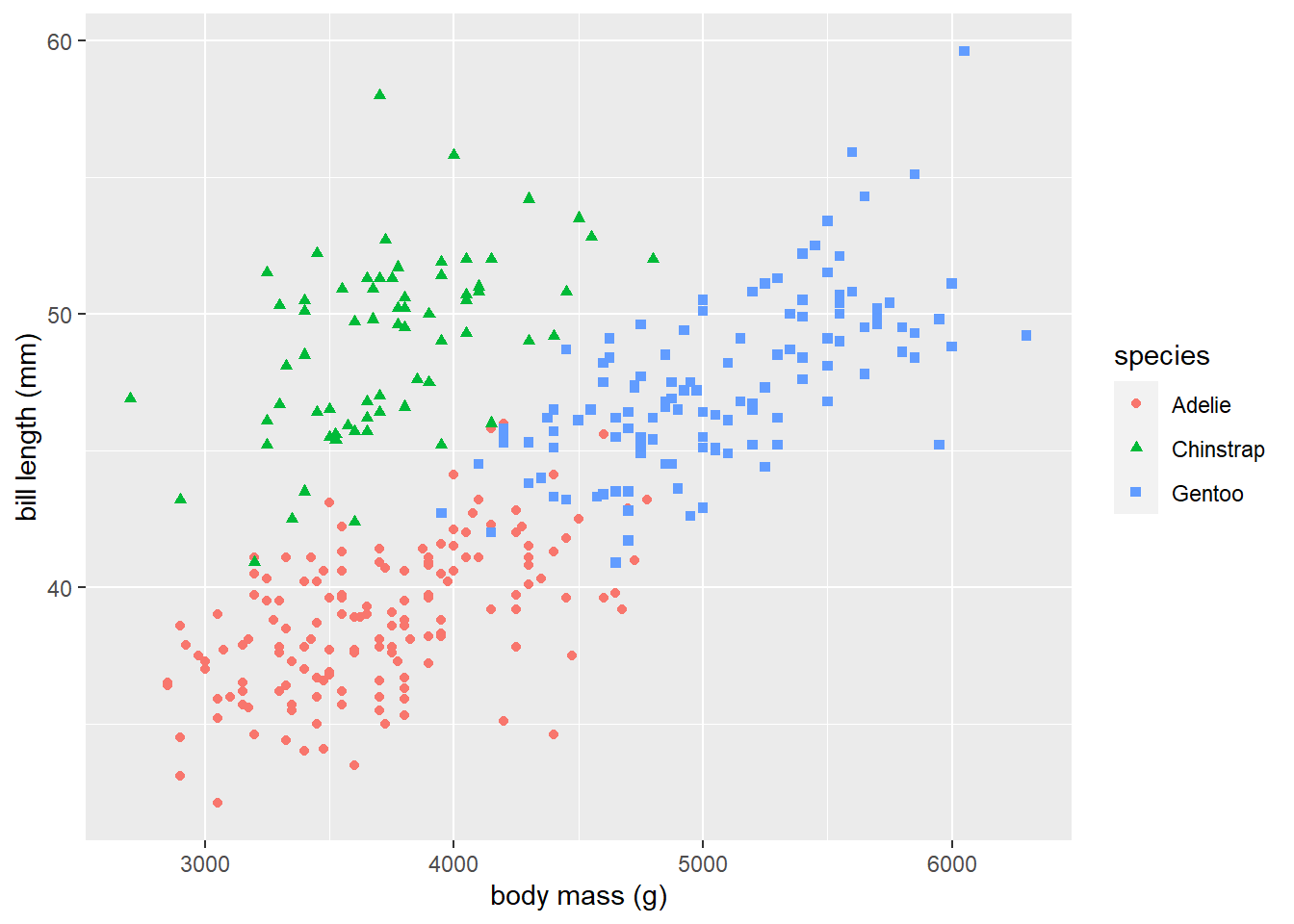

Figure 3.6: A grouped scatter plot of body mass versus bill length that distinguishes penguin species.

How do we use a categorical variable in R’s lm function? Recall that we should represent our categorical variables as a factor in R. The lm function will automatically convert a factor variable to the correct number of indicator variables when we include the factor variable in our formula argument. R will automatically choose the reference level to be the first level of the factor variable. To add a main effect term for a categorical predictor, we simply add the term to our lm formula. To create an interaction term, we use : between the interacting variables. E.g., if c is a factor variable and x is a numeric variable, we can use the notation c:x in our formula to get all the interactions between c and x.

In our present context, the categorical predictor of interest is species, which has the levels Adelie, Chinstrap, and Gentoo. The species variable is already a factor. Since the variable has 3 levels, it will be transformed into 2 indicator variables by R. The first level of species is Adelie, so R will treat that level as the reference level, and automatically create indicator variables for the levels Chinstrap and Gentoo. (Reminder: to determine the level order of a factor variable c, run the commend levels(c), or in this case levels(penguins$species).)

Let \(D_C\) denote the indicator variable for the Chinstrap level and \(D_G\) denote the indicator variable for the Gentoo level. To fit the parallel lines regression model \[E(\mathtt{bill\_length\_mm} \mid \mathtt{body\_mass\_g}, \mathtt{species}) = \beta_{0} + \beta_1 \mathtt{body\_mass\_g} + \beta_2 D_C + \beta_3 D_G,\] we run the code below. The coef function is used to extract the estimated coefficients from our fitted model in lmodp.

# fit parallel lines model
lmodp <- lm(bill_length_mm ~ body_mass_g + species, data = penguins)
# extract coefficients
coef(lmodp)
##      (Intercept)      body_mass_g speciesChinstrap 
##     24.919470977      0.003748497      9.920884113 
##    speciesGentoo 
##      3.557977539

Thus, the fitted parallel lines model is \[ \begin{aligned} &\hat{E}(\mathtt{bill\_length\_mm} \mid \mathtt{body\_mass\_g}, \mathtt{species}) \\ &= 24.92 + 0.004 \mathtt{body\_mass\_g} + 9.92 D_C + 3.56 D_G. \end{aligned} \tag{3.25} \] Note that speciesChinstrap and speciesGentoo are the indicator variables related to the Chinstrap and Gentoo levels of species, respectively, i.e., they represent \(D_C\) and \(D_G\). When an observation has species level Adelie, then Equation (3.25) simplifies to \[ \begin{aligned} &\hat{E}(\mathtt{bill\_length\_mm} \mid \mathtt{body\_mass\_g}, \mathtt{species}=\mathtt{Adelie}) \\ &=24.92 + 0.004 \mathtt{body\_mass\_g} + 9.92 \cdot 0 + 3.56 \cdot 0 \\ &= 24.92 + 0.004 \mathtt{body\_mass\_g}. \end{aligned} \] When an observation has species level Chinstrap, then Equation (3.25) simplifies to \[ \begin{aligned} &\hat{E}(\mathtt{bill\_length\_mm} \mid \mathtt{body\_mass\_g}, \mathtt{species}=\mathtt{Chinstrap}) \\ &=24.92 + 0.004 \mathtt{body\_mass\_g} + 9.92 \cdot 1 + 3.56 \cdot 0 \\ &= 34.84 + 0.004 \mathtt{body\_mass\_g}. \end{aligned} \] Lastly, when an observation has species level Gentoo, then Equation (3.25) simplifies to \[ \begin{aligned} &\hat{E}(\mathtt{bill\_length\_mm} \mid \mathtt{body\_mass\_g}, \mathtt{species}=\mathtt{Gentoo}) \\ &=24.92 + 0.004 \mathtt{body\_mass\_g} + 9.92 \cdot 0 + 3.56 \cdot 1 \\ &= 28.48 + 0.004 \mathtt{body\_mass\_g}. \end{aligned} \] Adding fitted lines for each species level to the scatter plot in Figure 3.6 is a bit more difficult than before. One technique is to use predict to get the fitted values of each observation, use the transform function to add those values as a column to the original the data frame, then use geom_line to connect the fitted values from each group.

We start by adding our fitted values to the penguins data frame. We use the predict function to obtained the fitted values of our fitted model and then use the transform function to add those values as the pl_fitted variable in the penguins data frame.

penguins <-
  penguins |>
  transform(pl_fitted = predict(lmodp))
## Error in data.frame(structure(list(species = structure(c(1L, 1L, 1L, 1L, : arguments imply differing number of rows: 344, 342

We just received a nasty error. What is going on? The original penguins data frame has 344 rows. However, two rows had NA observations such that when we used the lm function to fit our parallel lines model, those observations were removed prior to fitting. The predict function produces fitted values for the observations used in the fitting process, so there are only 342 predicted values. There is a mismatch between the number of rows in penguins and the number of values we attempt to add in the new column pl_fitted, so we get an error.

To handle this error, we refit our model while setting the na.action argument to na.exclude. As stated Details section of the documentation for the lm function (run ?lm in the Console):

\(\ldots\) when na.exclude is used the residuals and predictions are padded to the correct length by inserting NAs for cases omitted by na.exclude.

We refit the parallel lines model below with na.action = na.exclude, then use the predict function to add the fitted values to the penguins data frame via the transform function.

# refit parallel lines model with new na.action behavior
lmodp <- lm(bill_length_mm ~ body_mass_g + species, data = penguins, na.action = na.exclude)
# add fitted values to penguins data frame
penguins <-
  penguins |>
  transform(pl_fitted = predict(lmodp))

We now use the geom_line function to add the fitted lines for each species level to our scatter plot. Figure 3.7 displays the results from running the code below. The parallel lines model shown in Figure 3.7 fits the penguins data better than the simple linear regression model shown in Figure 3.5.

# create plot
# create scatterplot
# customize labels
# add lines for each level of species
ggplot(data = penguins) +
  geom_point(aes(x = body_mass_g, y = bill_length_mm,
                 shape = species, color = species)) +
  xlab("body mass (g)") + ylab("bill length (mm)") +
  geom_line(aes(x = body_mass_g, y = pl_fitted, color = species))

Figure 3.7: The fitted lines from the separate lines model for each level of species is added to the grouped scatter plot of bill_length_mm versus body_mass_g.

We now fit a separate lines regression model to the penguins data. Specifically, we fit the model \[ \begin{aligned} &E(\mathtt{bill\_length\_mm} \mid \mathtt{body\_mass\_g}, \mathtt{species}) \\ &= \beta_{0} + \beta_1 \mathtt{body\_mass\_g} + \beta_2 D_C + \beta_3 D_G + \beta_4 \mathtt{body\_mass\_g} D_C + \beta_5 \mathtt{body\_mass\_g} D_G , \end{aligned} \] using the code below, using the coef function to extract the estimated coefficients. The terms with : are interaction variables, e.g., body_mass_g:speciesChinstrap is \(\hat{\beta}_4\), the coefficient for the interaction between regressor \(\mathtt{body\_mass\_g} D_C\).

# fit separate lines model
# na.omit = na.exclude used to change predict behavior
lmods <- lm(bill_length_mm ~ body_mass_g + species + body_mass_g:species,
            data = penguins, na.action = na.exclude)
# extract estimated coefficients
coef(lmods)
##                  (Intercept)                  body_mass_g 
##                26.9941391367                 0.0031878758 
##             speciesChinstrap                speciesGentoo 
##                 5.1800537287                -0.2545906615 
## body_mass_g:speciesChinstrap    body_mass_g:speciesGentoo 
##                 0.0012748183                 0.0009029956

Thus, the fitted separate lines model is

\[ \begin{aligned} &\hat{E}(\mathtt{bill\_length\_mm} \mid \mathtt{body\_mass\_g}, \mathtt{species}) \\ &= 26.99 + 0.003 \mathtt{body\_mass\_g} + 5.18 D_C - 0.25 D_G \\ & \quad + 0.001 \mathtt{body\_mass\_g} D_C + 0.0009 \mathtt{body\_mass\_g} D_G. \end{aligned} \tag{3.26} \]

When an observation has species level Adelie, then Equation (3.26) simplifies to

\[ \begin{aligned} &\hat{E}(\mathtt{bill\_length\_mm} \mid \mathtt{body\_mass\_g}, \mathtt{species}=\mathtt{Adelie}) \\ &=26.99 + 0.003 \mathtt{body\_mass\_g} + 5.18 \cdot 0 - 0.25 \cdot 0\\ &\quad + 0.001 \cdot \mathtt{body\_mass\_g} \cdot 0 + 0.0009 \cdot \mathtt{body\_mass\_g} \cdot 0\\ &= 26.99 + 0.003 \mathtt{body\_mass\_g}. \end{aligned} \]

When an observation has species level Chinstrap, then Equation (3.26) simplifies to \[ \begin{aligned} &\hat{E}(\mathtt{bill\_length\_mm} \mid \mathtt{body\_mass\_g}, \mathtt{species}=\mathtt{Chinstrap}) \\ &=26.99 + 0.003 \mathtt{body\_mass\_g} + 5.18 \cdot 1 - 0.25 \cdot 0 \\ &\quad + 0.001 \cdot \mathtt{body\_mass\_g} \cdot 1 + 0.0009 \cdot \mathtt{body\_mass\_g} \cdot 0 \\ &= 31.17 + 0.004 \mathtt{body\_mass\_g}. \end{aligned} \] When an observation has species level Gentoo, then Equation (3.26) simplifies to \[ \begin{aligned} &\hat{E}(\mathtt{bill\_length\_mm} \mid \mathtt{body\_mass\_g}, \mathtt{species}=\mathtt{Chinstrap}) \\ &=26.99 + 0.003 \mathtt{body\_mass\_g} + 5.18 \cdot 0 - 0.25 \cdot 1 \\ &\quad + 0.001 \cdot \mathtt{body\_mass\_g} \cdot 0 + 0.0009 \cdot \mathtt{body\_mass\_g} \cdot 1 \\ &= 26.74 + 0.004 \mathtt{body\_mass\_g}. \end{aligned} \]

We use the code below to display the fitted lines for the separate lines model on the penguins data. Figure 3.8 shows the results. The fitted lines match the observed data behavior reasonably well.

# add separate lines fitted values to penguins data frame
penguins <-
  penguins |>
  transform(sl_fitted = predict(lmods))
# use geom_line to add fitted lines to plot
ggplot(data = penguins) +
  geom_point(aes(x = body_mass_g, y = bill_length_mm, shape = species, color = species)) +
  xlab("body mass (g)") + ylab("bill length (mm)") +
  geom_line(aes(x = body_mass_g, y = sl_fitted, col = species))

Figure 3.8: The fitted model for each level of species is added to the grouped scatter plot of bill_length_mm versus body_mass_g.

Having fit several models for the penguins data, we may be wondering how to evaluate how well the models fit the data. We discuss that in the next section.

3.10 Evaluating model fit

The most basic statistic measuring the fit of a regression model is the coefficient of determination, which is defined as \[ R^2 = 1 - \frac{\sum_{i=1}^n (Y_i-\hat{Y}_i)^2}{\sum_{i=1}^n (Y_i-\bar{Y})^2},\tag{3.27} \] where \(\bar{Y}\) is the sample mean of the observed response values.

To interpret this statistic, we need to introduce some new “sum-of-squares” statistics similar to the RSS.

The total sum of squares (corrected for the mean) is computed as \[ TSS = \sum_{i=1}^n(Y_i-\bar{Y})^2. \tag{3.28} \] The TSS is the sum of the squared deviations of the response values from the sample mean. However, it has a more insightful interpretation. Consider the constant mean model, which is the model \[ E(Y)=\beta_0. \tag{3.29} \] Using basic calculus, we can show that the OLS estimator of \(\beta_0\) for the model in Equation (3.29) is \(\hat{\beta}_0=\bar{Y}\). For the constant mean model, the fitted value of every observation is \(\hat{\beta}_0\), i.e., \(\hat{Y}_i=\hat{\beta}_0\) for \(i=1,2,\ldots,n\). Thus, the RSS of the constant mean model is \(\sum_{i=1}^n(Y_i-\hat{Y}_i)^2=\sum_{i=1}^n(Y_i-\bar{Y})^2\). Thus, the TSS is the RSS for the constant mean model.

The regression sum-of-squares or model sum-of-squares is defined as \[ SS_{reg} = \sum_{i=1}^n(\hat{Y}_i-\bar{Y})^2. \tag{3.30} \] Thus, SS_reg is the sum of the squared deviations between the fitted values of a model and the fitted values of the constant mean model. More helpfully, we have the following equation relating TSS, RSS, and SS_reg: \[ TSS = RSS + SS_{reg}.\tag{3.31} \] Thus, \(SS_{reg}=TSS-RSS\). This means that SS_reg measures the reduction in RSS when comparing the fitted model to the constant mean model.

Comparing Equations (3.6), (3.27), (3.28), and (3.30), we can express \(R^2\) as: \[ \begin{aligned} R^2 &= 1-\frac{\sum_{i=1}^n (Y_i-\hat{Y}_i)^2}{\sum_{i=1}^n (Y_i-\bar{Y})^2} \\ &= 1 - \frac{RSS}{TSS} \\ &= \frac{TSS - RSS}{TSS} \\ &= \frac{SS_{reg}}{TSS} \\ &= [\mathrm{cor}(\mathbf{y}, \hat{\mathbf{y}})]^2. \end{aligned} \tag{3.32} \] The last expression is the squared sample correlation between the observed and fitted values, and is a helpful way to express the coefficient of determination because it extends to regression models that are not linear.

Looking at Equation (3.32) in particular, we can say that the coefficient of determination is the proportional reduction in RSS when comparing the fitted model to the constant mean model.

Some comments about the coefficient of determination:

• \(0\leq R^2 \leq 1\).
• \(R^2=0\) for the constant mean model.
• \(R^2=1\) for a fitted model that perfectly fits the data (the fitted values match the observed response values).
• Generally, larger values of \(R^2\) suggest that the model explains a lot of the variation in the response variable. Smaller \(R^2\) values suggest the fitted model does not explain a lot of the response variation.
• The Multiple R-squared value printed by the summary of an lm object is \(R^2\).
• To extract \(R^2\) from a fitted model, we can use the syntax summary(lmod)$r.squared, where lmod is our fitted model.

Figure 3.9 provides examples of the \(R^2\) value for various fitted simple linear regression models. The closer the points fall to a straight line, the larger \(R^2\) tends to be. However, as shown in the bottom right panel of Figure 3.9, a poorly fit model can result in a lower \(R^2\) model even if there is a clear relationship between the points (the points have a perfect quadratic relationship).

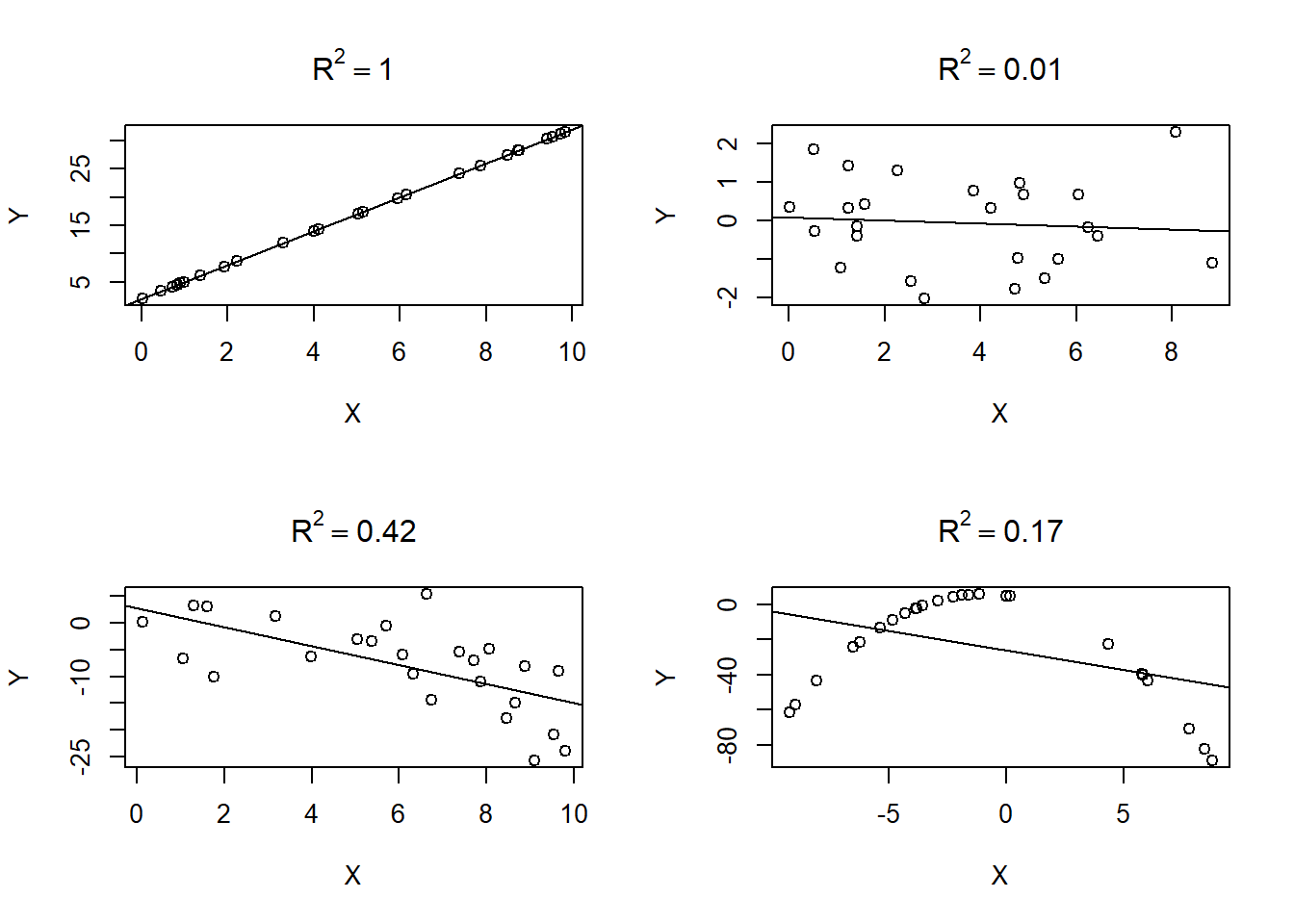
Figure 3.9: The coefficient of determination values for 4 different data sets.

The coefficient of determination for the parallel lines model fit to the penguins data in Section 3.9 is 0.81, as shown in the R output below. By adding the body_mass_g regressor and species predictor to the constant mean model of bill_length_mm, we reduced the RSS by 81%.

summary(lmodp)$r.squared
## [1] 0.8079566

It may seem sensible to choose between models based on the value of \(R^2\). This is unwise for two reasons:

1. \(R^2\) never decreases as regressors are added to an existing model. Basically, we can increase \(R^2\) by simply adding regressors to our existing model, even if they are non-sensical.
2. \(R^2\) doesn’t tell us whether a model adequately describes the pattern of the observed data. \(R^2\) is a useful statistic for measuring model fit when there is approximately a linear relationship between the response values and fitted values.

Regarding point 1, consider what happens when we add a regressor of random values to the parallel lines model fit to the penguins data. The code below sets a random number seed so that we can get the same results each time we run the code, creates the regressor noisyx by sampling 344 values randomly drawn from a \(\mathcal{N}(0,1)\) distribution, adds noisyx as a regressor to the parallel lines regression model stored in lmodp, and then extracts the \(R^2\) value. We use the update method to update our existing model. The update function takes an existing model as its first argument and then the formula for the updated model. The syntax . ~ . means “keep the same response (on the left) and the same regressors (on the right)”. We can then add or subtract regressors using the typical formula syntax. We use this approach to add the noisyx regressor to the regressors already in lmodp.

set.seed(28) # for reproducibility
# create regressor of random noise
noisyx <- rnorm(344)
# add noisyx as regressor to lmodp
lmod_silly <- update(lmodp, . ~ . + noisyx)
# extract R^2 from fitted model
summary(lmod_silly)$r.squared
## [1] 0.8087789

The \(R^2\) value increased from 0.8080 to 0.8088! So clearly, choosing the model with the largest \(R^2\) can be a mistake, as it will tend to favor models with more regressors.

Regarding point 2, \(R^2\) can mislead us into thinking an inappropriate model fits better than it actually does. Anscombe (1973) provided a canonical data set known as “Anscombe’s quartet” that illustrates this point. The data set is comprised of 4 different data sets. When a simple linear regression model is fit to each data set, we find that \(\hat{\beta}_0=3\), \(\hat{\beta}_1=0.5\), and that \(R^2=0.67\). However, as we will see, not all models describe the data particularly well!

Anscombe’s quartet is available as the anscombe data set in the datasets package. The data set includes 11 observations of 8 variables. The variables are:

• x1, x2, x3, x4: the regressor variable for each individual data set.
• y1, y2, y3, y4: the response variable for each individual data set.

We fit the simple linear regression model to the four data sets in the code below, then extract the coefficients and \(R^2\) to verify the information provided above.

# fit model to first data set
lmod_a1 <- lm(y1 ~ x1, data = anscombe)
# extract coefficients from fitted model
coef(lmod_a1)
## (Intercept)          x1 
##   3.0000909   0.5000909
# extract R^2 from fitted model
summary(lmod_a1)$r.squared
## [1] 0.6665425
# fit model to second data set
lmod_a2 <- lm(y2 ~ x2, data = anscombe)
coef(lmod_a2)
## (Intercept)          x2 
##    3.000909    0.500000
summary(lmod_a2)$r.squared
## [1] 0.666242
# fit model to third data set
lmod_a3 <- lm(y3 ~ x3, data = anscombe)
coef(lmod_a3)
## (Intercept)          x3 
##   3.0024545   0.4997273
summary(lmod_a3)$r.squared
## [1] 0.666324
# fit model to fourth data set
lmod_a4 <- lm(y4 ~ x4, data = anscombe)
coef(lmod_a4)
## (Intercept)          x4 
##   3.0017273   0.4999091
summary(lmod_a4)$r.squared
## [1] 0.6667073

Figure 3.10 provides a scatter plot each data set and overlays their fitted models.

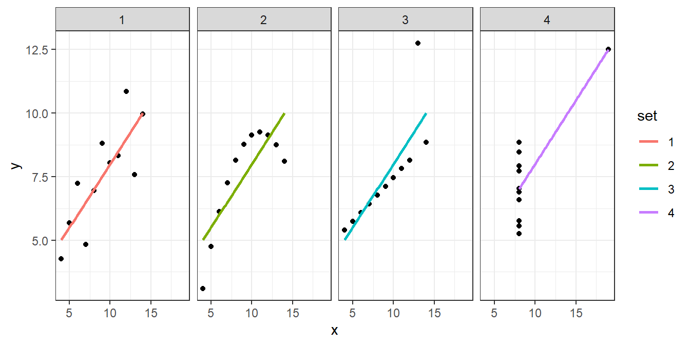
Figure 3.10: Scatter plots of the four Anscombe data sets along with their line of best fit.

While the fitted model and \(R^2\) value is essentially the same for each model, the fitted model is only appropriate for data set 1. The fitted model for the second data set fails to model the curve of the data. The third fitted model doesn’t handle the outlier in the data. Lastly, the fourth data set has a single point on the far right side driving the model fit, so the fitted model is highly questionable.

To address the problem with \(R^2\) that it cannot decrease as regressors are added to a model, Ezekiel (1930) proposed the adjusted R-squared statistic for measuring model fit. The adjusted \(R^2\) statistic is defined as \[ R^2_a=1-(1-R^2)\frac{n-1}{n-p}=1-\frac{RSS/(n-p)}{TSS/(n-1)}. \] Practically speaking, \(R^2_a\) will only increase when a regressors substantively improves the fit of the model to the observed data. We favor models with larger values of \(R^2_a\). To extract the adjusted R-squared from a fitted model, we can use the syntax summary(lmod)$adj.R.squared, where lmod is the fitted model.

Using the code below, we extract the \(R^2_a\) for the 4 models we previously fit to the penguins data. Specifically, we extract \(R_a^2\) for the simple linear regression model fit in Section 3.3, the multiple linear regression model in Section 3.6, and the parallel and separate lines models fit in Section 3.9.

# simple linear regression model
summary(lmod)$adj.r.squared
## [1] 0.3522562
# multiple linear regression model
summary(mlmod)$adj.r.squared
## [1] 0.4295084
# parallel lines model
summary(lmodp)$adj.r.squared
## [1] 0.8062521
# separate lines model
summary(lmods)$adj.r.squared
## [1] 0.8069556

With an \(R_a^2\) of 0.8070, the separate lines regression model appears to be slightly favored over the other 3 models fit to the penguins data. To confirm that this statistic is meaningful (i.e., that the model provides a reasonable fit to the data), we use the code below to create a scatter plot of the response versus fitted values shown in Figure 3.11. The points in Figure 3.11 follow a linear pattern, so the separate lines model seems to be a reasonable model for the penguins data.

plot(penguins$bill_length_mm ~ fitted(lmods),
     xlab = "fitted values", ylab = "bill length (mm)")

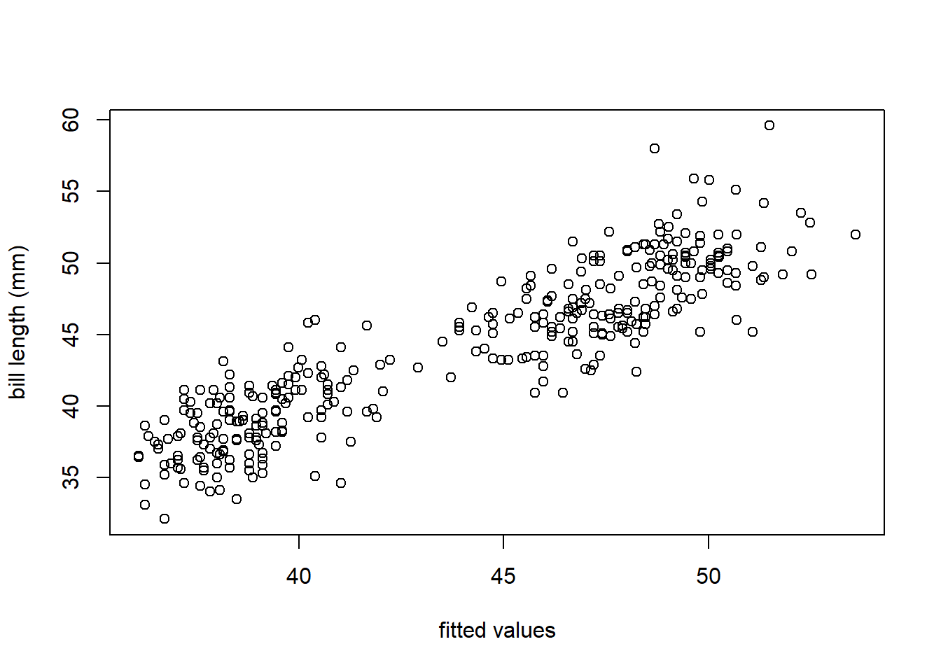
Figure 3.11: A scatter plot of the observed bill length versus the fitted values of the separate lines model for the penguins data.

3.11 Summary

In this chapter, we learned:

• What a linear model is.
• What various objects are, such as coefficients, residuals, fitted values, etc.
• How to estimate the coefficients of a linear model using ordinary least squares estimation.
• How to fit a linear model using R.
• How to include a categorical predictor in a linear model.
• How to evaluate the fit of a model.

3.11.1 Summary of terms

We have introduced many terms to define a linear model. It can be difficult to keep track of their notation, their purpose, whether they are observable, and whether they are treated as random variables or vectors. We discuss various terms below, and then summarize the discussion in Table 3.2.

We’ve already talked about observing the response variable and the predictor/regressor variables. So these objects are observable. However, we have no way to measure the regression coefficients or the error. These are not observable. One way to distinguish observable versus non-observable variables is that observable variables are denoted using Phoenician letters (e.g., \(X\) and \(Y\)) while non-observable variables are denoted using Greek letters (e.g., \(\beta_j\), \(\epsilon\), \(\sigma^2\)).

We treat the response variable as a random variable. Perhaps surprisingly, we treat the predictor and regressor variables as fixed, non-random variables. The regression coefficients are treated as fixed, non-random but unknown values. This is standard for parameters in a statistical model. The errors are also treated as random variables. In fact, since both the regressor variables and the regression coefficients are non-random, the only way for the responses in Equation (3.14) to be random variables is for the errors to be random.

Table 3.2: An overview of terms used to define a linear model.

Term	Description	Observable?	Random?
\(Y\)	response variable	Yes	Yes
\(Y_i\)	response value for the \(i\)th observation	Yes	Yes
\(\mathbf{y}\)	the \(n\times 1\) column vector of response values	Yes	Yes
\(X\)	regressor variable	Yes	No
\(X_j\)	the \(j\)th regressor variable	Yes	No
\(x_{i,j}\)	the value of the \(j\)th regressor variable for the \(i\)th observation	Yes	No
\(\mathbf{X}\)	the \(n\times p\) matrix of regressor values	Yes	No
\(\mathbf{x}_i\)	the \(p\times 1\) vector of regressor values for the \(i\)th observation	Yes	No
\(\beta_j\)	the coefficient associated with the \(j\)th regressor variable	No	No
\(\boldsymbol{\beta}\)	the \(p\times 1\) column vector of regression coefficients	No	No
\(\epsilon\)	the model error	No	Yes
\(\epsilon_i\)	the error for the \(i\)th observation	No	Yes
\(\boldsymbol{\epsilon}\)	the \(n\times 1\) column vector of errors	No	Yes

3.11.2 Summary of functions

We have used many functions in this Chapter. We summarize some of the most important ones in Table 3.3.

Table 3.3: An overview of important functions discussed in this chapter.

Function	Purpose
lm	Fits a linear model based on a provided formula
summary	Provides summary information about the fitted model
coef	Extracts the vector of estimated regression coefficients from the fitted model
residuals	Extracts the vector of residuals from the fitted model
fitted	Extracts the vector of fitted values from the fitted model
predict	Computes the fitted values (or arbitrary predictions) based on a fitted model
deviance	Extracts the RSS of a fitted model
sigma	Extracts \(\hat{\sigma}\) from the fitted model
update	Updates a fitted model to remove or add regressors

3.12 Going Deeper

3.12.1 Degrees of freedom

The degrees of freedom of a statistics refers to the number of independent pieces of information that go into its calculation.

Consider the sample mean \[\bar{x}=\sum_{i=1}^n x_i.\]

The calculation uses \(n\) pieces of information to compute, but the statistic only has \(n-1\) degrees of freedom. Once we know the sample mean, only \(n-1\) values are independent, while the last is constrained to be a certain value.

Let’s say \(n=3\) and \(\bar{x} = 10\). Then \(x_1\) and \(x_2\) can be any numbers, but the last value MUST equal \(30 - x_1 - x_2\) so that \(x_1 + x_2 + x_3 = 30\) (otherwise the sample mean won’t equal 10). To be more specific, if \(x_1 = 5\) and \(x_2 = 25\), then \(x_3\) must be 0, otherwise the sample mean won’t be 10.

3.12.2 Derivation of the OLS estimators of the simple linear regression model coefficients

Assume a simple linear regression model with \(n\) observations. The residual sum of squares for the simple linear regression model is \[ RSS(\hat\beta_0, \hat\beta_1) = \sum_{i=1}^n(Y_i - \hat\beta_0 - \hat\beta_1x_i)^2. \]

OLS estimator of \(\beta_0\)

First, we take the partial derivative of the RSS with respect to \(\hat\beta_0\) and simplify: \[ \begin{aligned} \frac{\partial RSS(\hat\beta_0, \hat\beta_1)}{\partial \hat\beta_0} &= \frac{\partial}{\partial \hat\beta_0}\sum_{i=1}^n(Y_i - \hat\beta_0 - \hat\beta_1x_i)^2 & \tiny\text{ (substituting the formula for the RSS)} \\ &= \sum_{i=1}^n \frac{\partial}{\partial \hat\beta_0}(Y_i - \hat\beta_0 - \hat\beta_1x_i)^2 & \tiny\text{ (by the linearity property of derivatives)} \\ &= -2\sum_{i=1}^n(Y_i - \hat\beta_0 - \hat\beta_1x_i). & \tiny\text{ (chain rule, factoring out -2)} \end{aligned} \]

Next, we set the partial derivative equal to zero and rearrange the terms to solve for \(\hat{\beta}_0\): \[ \begin{aligned} 0 &= \frac{\partial RSS(\hat\beta_0, \hat\beta_1)}{\partial \hat\beta_0} & \\ 0 &= -2\sum_{i=1}^n(Y_i - \hat\beta_0 - \hat\beta_1x_i) & \tiny\text{ (substitute partial deriviative)}\\ 0 &= \sum_{i=1}^n(Y_i - \hat\beta_0 - \hat\beta_1x_i) & \tiny\text{ (divide both sides by -2)} \\ 0 &= \sum_{i=1}^n Y_i - \sum_{i=1}^n\hat\beta_0 - \sum_{i=1}^n\hat\beta_1x_i &\tiny\text{ (by linearity of sum)} \\ 0 &= \sum_{i=1}^n Y_i - n\hat\beta_0 - \sum_{i=1}^n\hat\beta_1x_i & \tiny(\text{sum }\hat\beta_0\ n\text{ times equals }n\hat\beta_0) \\ n\hat\beta_0 &= \sum_{i=1}^n Y_i-\hat{\beta}_1\sum_{i=1}^nx_i. &\tiny\text{ (algebra rearrange, factor }\hat{\beta}_1\text{)} \\ \end{aligned} \]

Finally, we divide both sides by \(n\) to get the OLS estimator for \(\hat\beta_0\) in terms of \(\hat\beta_1\): \[ \hat\beta_0 = \bar Y-\hat\beta_1\bar x \]

OLS Estimator of \(\beta_1\)

Similar to the previous derivation, we differentiate the RSS with respect to the parameter estimate of interest, set the derivative equal to zero, and solve for the parameter.

We start by taking the partial derivative of the RSS with respect to \(\hat{\beta}_1\) and simplify. \[ \begin{aligned} \frac{\partial RSS(\hat\beta_0, \hat\beta_1)}{\partial \hat\beta_1} &= \frac{\partial}{\partial \hat\beta_1}\sum_{i=1}^n (Y_i - \hat\beta_0 - \hat\beta_1x_i)^2 & \tiny\text{ (substitute formula for RSS)} \\ &= \sum_{i=1}^n \frac{\partial}{\partial \hat\beta_1}(Y_i - \hat\beta_0 - \hat\beta_1x_i)^2 & \tiny\text{ (linearity property of derivatives)} \\ &= -2\sum_{i=1}^n(Y_i-\hat\beta_0-\hat\beta_1x_i)x_i & \tiny\text{ (chain rule, factor out -2)} \end{aligned} \]

We now set this derivative equal to 0 and rearrange the terms to solve for \(\hat{\beta}_1\): \[ \begin{aligned} 0 &= \frac{\partial RSS(\hat\beta_0, \hat\beta_1)}{\partial \hat\beta_1} & \\ 0 &= -2\sum_{i=1}^n(Y_i-\hat\beta_0-\hat\beta_1x_i)x_i &\tiny\text{(substitute partial derivative})\\ 0 &= \sum_{i=1}^n(Y_i-(\bar Y -\hat \beta_1\bar x)-\hat\beta_1x_i)x_i &\tiny\text{(substitute OLS estimator of }\hat\beta_0, \text{ divide both sides by -2}) \\ 0 &= \sum_{i=1}^n x_iY_i -\sum_{i=1}^n x_i\bar Y+\hat\beta_1\bar x\sum_{i=1}^n x_i-\hat\beta_1\sum_{i=1}^n x_i^2. &\tiny\text{(expand sum, use linearity of sum)} \\ \end{aligned} \]

Continuing from the previous line, we move the terms involving \(\hat{\beta}_1\) to the other side of the equality to get \[ \begin{aligned} \hat\beta_1\sum_{i=1}^n x_i^2-\hat\beta_1\bar x\sum_{i=1}^n x_i &=\sum_{i=1}^n x_iY_i -\sum_{i=1}^n x_i\bar Y & \tiny\text{(move estimator to other side)}\\ \hat\beta_1\sum_{i=1}^n x_i^2-\hat\beta_1\frac{1}{n}\sum_{i=1}^n x_i\sum_{i=1}^n x_i&=\sum_{i=1}^n x_iY_i -\sum_{i=1}^n x_i\frac{1}{n}\sum_{i=1}^n Y_i &\tiny\text{(rewrite using definition of sample means)} \\ \hat\beta_1\sum_{i=1}^n x_i^2-\hat\beta_1\frac{1}{n}\left(\sum_{i=1}^n x_i\right)^2 &=\sum_{i=1}^n x_iY_i -\frac{1}{n}\sum_{i=1}^n x_i\sum_{i=1}^n Y_i & \tiny\text{(reorder and simplify)} \\ \hat\beta_1\left(\sum_{i=1}^n x_i^2-\frac{1}{n}\left(\sum_{i=1}^n x_i\right)^2\right)&=\sum_{i=1}^n x_iY_i -\frac{1}{n}\sum_{i=1}^n x_i\sum_{i=1}^n Y_i, & \tiny\text{(factoring)}\\ \end{aligned} \] which allows us to obtain \[ \hat\beta_1=\frac{\sum_{i=1}^n x_iY_i -\frac{1}{n}\sum_{i=1}^n x_i\sum_{i=1}^n Y_i}{\sum_{i=1}^n x_i^2-\frac{1}{n}\left(\sum_{i=1}^n x_i\right)^2}. \]

Thus, we have the OLS estimators of the simple linear regression coefficients are \[ \begin{aligned} \hat\beta_0 &= \bar Y-\hat\beta_1\bar x, \\ \hat\beta_1 & =\frac{\sum_{i=1}^n x_iY_i -\frac{1}{n}\sum_{i=1}^n x_i\sum_{i=1}^n Y_i}{\sum_{i=1}^n x_i^2-\frac{1}{n}\left(\sum_{i=1}^n x_i\right)^2}. \end{aligned} \]

3.12.3 Unbiasedness of OLS estimators

We now show that the OLS estimators we derived in Section 3.12.2 are unbiased. An estimator is unbiased if the expected value is equal to the parameter it is estimating.

The OLS estimator assumes we know the value of the regressor variables for all observations. Thus, we must condition our expectation on knowing the regressor matrix \(\mathbf{X}\). Thus, we want to show that \[ E(\hat{\beta}_0\mid \mathbf{X})=\beta_0, \] where “\(\mid \mathbf{X}\)” is convenient notation to indicate that we are conditioning our expectation on knowing the regressor values for every observation.

In Section 3.2, we noted that we assume \(E(\epsilon \mid X)=0\), which is true for every error in our model, i.e. \(E(\epsilon_i \mid X = x_i) = 0\) for \(i=1,2,\ldots,n\). Thus,

\[ \begin{aligned} E(Y_i\mid X=x_i) &= E(\beta_0 + \beta_1 x_i +\epsilon_i\mid X = x_i) & \tiny\text{(substiute definition of $Y_i$)} \\ &= E(\beta_0\mid X=x_i) + E(\beta_1 x_i \mid X = X_i) +E(\epsilon_i | X=x_i) & \tiny\text{(linearity property of expectation)} \\ &= \beta_0+\beta_1x_i +E(\epsilon_i | X=x_i) & \tiny\text{(the $\beta$s and $x_i$ are non-random values)} \\ &= \beta_0+\beta_1x_i + 0 & \tiny\text{(assumption about errors)} \\ &= \beta_0+\beta_1x_i. & \end{aligned} \]

In the derivations below, every sum is over all values of \(i\), i.e., \(\sum \equiv \sum_{i=1}^n\). We drop the index for simplicity.

Next, we note: \[ \begin{aligned} E\left(\sum x_iY_i \biggm| \mathbf{X} \right) &= \sum E(x_iY_i \mid \mathbf{X}) &\tiny\text{ (by the linearity of the expectation operator)}\\ &=\sum x_iE(Y_i\mid \mathbf{X})&\tiny(x_i\text{ is a fixed value, so it can be brought out})\\ &=\sum x_i(\beta_0+\beta_1 x_i)&\tiny\text{(substitute expected value of }Y_i)\\ &=\sum x_i\beta_0+\sum x_i\beta_1 x_i&\tiny\text{(distribute sum)}\\ &=\beta_0\sum x_i+\beta_1\sum x_i^2.&\tiny\text{(factor out constants)} \end{aligned} \]

Also, \[ \begin{aligned} E(\bar Y\mid \mathbf{X}) &= E\left(\frac{1}{n}\sum Y_i\Biggm|\mathbf{X} \right)&\tiny\text{(definition of sample mean)}\\ &= \frac{1}{n}E\left(\sum Y_i \Bigm| \mathbf{X}\right)&\tiny\text{(factor out constant)}\\ &= \frac{1}{n}\sum E\left(Y_i \mid \mathbf{X}\right)&\tiny\text{(linearity of expectation)}\\ &= \frac{1}{n}\sum(\beta_0+\beta_1 x_i)&\tiny\text{(substitute expected value of }Y_i)\\ &= \frac{1}{n}\left(\sum\beta_0+\sum\beta_1 x_i\right)&\tiny\text{(distribute sum)}\\ &= \frac{1}{n}\left(n\beta_0+\beta_1\sum x_i\right)&\tiny\text{(simplify, factor out constant)}\\ &= \beta_0+\beta_1\bar x. &\tiny\text{(simplify)} \end{aligned} \]

To simplify our derivation below, define \[ SSX = \sum x_i^2-\frac{1}{n}\left(\sum x_i\right)^2. \] Thus,

\[ \begin{aligned} &E(\hat\beta_1 \mid \mathbf{X}) &\\ &= E\left(\frac{\sum x_iY_i -\frac{1}{n}\sum x_i\sum Y_i}{\sum x_i^2-\frac{1}{n}\left(\sum x_i\right)^2} \Biggm| \mathbf{X} \right) &\tiny\text{(substitute OLS estimator)} \\ &= \frac{1}{SSX}E\left(\sum x_iY_i-\frac{1}{n}\sum x_i\sum Y_i \biggm| \mathbf{X}\right)&\tiny\text{(factor out constant denominator, substitute }SSX\text{)} \\ &= \frac{1}{SSX}\left[E\left(\sum x_iY_i\Bigm|\mathbf{X}\right)-E\left(\frac{1}{n}\sum x_i\sum Y_i\biggm|\mathbf{X}\right)\right]&\tiny\text{(linearity of expectation)}\\ &= \frac{1}{SSX}\left[E\left(\sum x_iY_i\Bigm|\mathbf{X}\right)-\left(\sum x_i\right)E\left(\bar Y\mid \mathbf{X}\right)\right]&\tiny\text{(factor out constant }\sum x_i\text{, use definition of}\bar{Y})\\ &= \frac{1}{SSX}\left[\left(\beta_0\sum x_i + \beta_1\sum x_i^2\right)-\left(\sum x_i\right)(\beta_0+\beta_1\bar x)\right]&\tiny\text{(substitute previous derivations )}\\ &= \frac{1}{SSX}\left[\beta_0\sum x_i+\beta_1\sum x_i^2-\beta_0\sum x_i-\beta_1\bar x\sum x_i\right]&\tiny\text{(expand product and reorder)} \\ &= \frac{1}{SSX}\left[\beta_1\sum x_i^2-\beta_1\bar x\sum x_i\right]&\tiny\text{(cancel terms)}\\ &= \frac{1}{SSX}\left[\beta_1\sum x_i^2-\beta_1\frac{1}{n}\sum x_i\sum x_i\right]&\tiny\text{(using definition of sample mean)}\\ &= \frac{1}{SSX}\beta_1\left[\sum x_i^2-\frac{1}{n}\left(\sum x_i\right)^2\right]&\tiny\text{(factor out }\beta_1\text{, simplify})\\ &= \frac{1}{SSX}\beta_1[SSX]&\tiny\text{(substitute }SSX\text{)} \\ &=\beta_1. &\tiny\text{(simplify)} \end{aligned} \]

Therefore, \(\hat\beta_1\) is an unbiased estimator of \(\beta_1\).

Next, we show that \(\hat\beta_0\) is unbiased: \[ \begin{aligned} E(\hat\beta_0\mid \mathbf{X}) &= E(\bar Y - \hat{\beta}_1\bar x\mid \mathbf{X}) &\tiny\text{(OLS estimator of }\beta_0) \\ &= E(\bar{Y}\mid \mathbf{X}) - E(\hat\beta_1\bar{x}\mid \mathbf{X}) &\tiny\text{(linearity of expectation})\\ &= E(\bar{Y}\mid \mathbf{X}) - \bar{x}E(\hat\beta_1\mid \mathbf{X}) &\tiny\text{(factor out constant})\\ &= \beta_0 +\beta_1\bar x-\bar x\beta_1 &\tiny\text{(substitute previous derivations})\\ &= \beta_0. &\tiny\text{(cancel terms})\\ \end{aligned} \]

Therefore, \(\hat\beta_0\) is an unbiased estimator of \(\beta_0\).

3.12.4 Manual calculation Penguins simple linear regression example

In this section, we manually produce (i.e., without the lm function) the penguins simple linear regression example in Section 3.3.

First, we will manually fit a simple linear regression model that regresses bill_length_mm on body_mass_g.

Using the summary function on the penguins data frame, we see that both bill_length_mm and body_mass_g have NA values.

summary(penguins)
##       species          island    bill_length_mm 
##  Adelie   :152   Biscoe   :168   Min.   :32.10  
##  Chinstrap: 68   Dream    :124   1st Qu.:39.23  
##  Gentoo   :124   Torgersen: 52   Median :44.45  
##                                  Mean   :43.92  
##                                  3rd Qu.:48.50  
##                                  Max.   :59.60  
##                                  NA's   :2      
##  bill_depth_mm   flipper_length_mm  body_mass_g  
##  Min.   :13.10   Min.   :172.0     Min.   :2700  
##  1st Qu.:15.60   1st Qu.:190.0     1st Qu.:3550  
##  Median :17.30   Median :197.0     Median :4050  
##  Mean   :17.15   Mean   :200.9     Mean   :4202  
##  3rd Qu.:18.70   3rd Qu.:213.0     3rd Qu.:4750  
##  Max.   :21.50   Max.   :231.0     Max.   :6300  
##  NA's   :2       NA's   :2         NA's   :2     
##      sex           year        pl_fitted    
##  female:165   Min.   :2007   Min.   :35.60  
##  male  :168   1st Qu.:2007   1st Qu.:38.98  
##  NA's  : 11   Median :2008   Median :45.67  
##               Mean   :2008   Mean   :43.92  
##               3rd Qu.:2009   3rd Qu.:48.34  
##               Max.   :2009   Max.   :52.83  
##                              NA's   :2      
##    sl_fitted    
##  Min.   :36.08  
##  1st Qu.:38.95  
##  Median :45.40  
##  Mean   :43.92  
##  3rd Qu.:48.42  
##  Max.   :53.60  
##  NA's   :2

This is important to note because the lm function automatically removes any observation with NA values for any of the variables specified in the formula argument. In order to replicate our results, we must remove the same observations.

We want to remove the rows of penguins where either body_mass_g or bill_length_mm have NA values. We do that below using the na.omit function (selecting only the relevant variables) and assign the cleaned object the name penguins_clean.

# remove rows of penguins where bill_length_mm or body_mass_g have NA values
penguins_clean <-
  penguins |>
  subset(select = c("bill_length_mm", "body_mass_g")) |>
  na.omit()

We extract the bill_length_mm variable from the penguins data frame and assign it the name y since it will be the response variable. We extract the body_mass_g variable from the penguins data frame and assign it the name x since it will be the regressor variable. We also determine the number of observations and assign that value the name n.

# extract response and regressor from penguins_clean
y <- penguins_clean$bill_length_mm
x <- penguins_clean$body_mass_g
# determine number of observations
n <- length(y)

We now compute \(\hat{\beta}_1\) and \(\hat{\beta}_0\) using Equations (3.9) and (3.10). Note that placing () around the assignment operations will both perform the assignment and print the results.

# compute OLS estimate of beta1
(b1 <- (sum(x * y) - sum(x) * sum(y) / n)/(sum(x^2) - sum(x)^2/n))
## [1] 0.004051417
# compute OLS estimate of beta0
(b0 <- mean(y) - b1 * mean(x))
## [1] 26.89887

The estimated value of \(\beta_0\) is \(\hat{\beta}_0=26.90\) and the estimated value of \(\beta_1\) is \(\hat{\beta}_1=0.004\).

We can also compute the residuals, the fitted values, the RSS, and the estimated error variance. Using the code below, the RSS for our model is 6564.49 and the estimated error variance if \(\hat{\sigma}^2=19.31\).

yhat <- b0 + b1 * x # compute fitted values
ehat <- y - yhat # compute residuals
(rss <- sum(ehat^2)) # sum of the squared residuals
## [1] 6564.494
(sigmasqhat <- rss/(n-2)) # estimated error variance
## [1] 19.30734

3.12.5 Derivation of the OLS estimator for the multiple linear regression model coefficients

We want to determine the value of \(\hat{\boldsymbol{\beta}}\) that will minimize \[ \begin{aligned} RSS(\hat{\boldsymbol{\beta}}) &=\sum_{i=1}^n \hat{\epsilon_i}^2 \\ &= \hat{\boldsymbol{\epsilon}}^T\hat{\boldsymbol{\epsilon}} \\ &= (\mathbf{y} - \mathbf{X}\hat{\boldsymbol{\beta}})^T(\mathbf{y} - \mathbf{X}\hat{\boldsymbol{\beta}}) \\ &= \mathbf{y}^T\mathbf{y}-2\hat{\boldsymbol{\beta}}^T\mathbf{X}^T\mathbf{y}+\hat{\boldsymbol{\beta}}^T\mathbf{X}^T\mathbf{X}\hat{\boldsymbol{\beta}}, \end{aligned} \] where the second term in the last line comes from the fact that \(\hat{\boldsymbol{\beta}}^T\mathbf{X}^T\mathbf{y}\) is a \(1\times 1\) matrix, and is thus symmetric. Consequently, \(\hat{\boldsymbol{\beta}}^T\mathbf{X}^T\mathbf{y}=(\hat{\boldsymbol{\beta}}^T\mathbf{X}^T\mathbf{y})^T=\mathbf{y}^T\mathbf{X}\hat{\boldsymbol{\beta}}\).

To find the local extrema of \(RSS(\hat{\boldsymbol{\beta}})\), we set its derivative with respect to \(\hat{\boldsymbol{\beta}}\) equal to 0, and solve for \(\hat{\boldsymbol{\beta}})\).

Using the results in Appendix A.5, we see that \[ \frac{\partial RSS(\hat{\boldsymbol{\beta}})}{\partial\hat{\boldsymbol{\beta}}} = -2\mathbf{X}^T\mathbf{y} + 2\mathbf{X}^T\mathbf{X}\hat{\boldsymbol{\beta}}. \] Setting \(\partial RSS(\hat{\boldsymbol{\beta}})/\partial\hat{\boldsymbol{\beta}}=0\) and using some simple algebra, we derive the normal equations \[\mathbf{X}^T\mathbf{X}\hat{\boldsymbol{\beta}}=\mathbf{X}^T\mathbf{y}.\] Assuming the \(\mathbf{X}^T\mathbf{X}\) is invertible, which it will be when \(\mathbf{X}\) is full-rank, our solution is \[\hat{\boldsymbol{\beta}}=(\mathbf{X}^T\mathbf{X})^{-1}\mathbf{X}^T\mathbf{y}.\]

To show that the OLS estimator of \(\boldsymbol{\beta}\) minimizes \(RSS(\hat{\boldsymbol{\beta}})\), we technically need to show that the Hessian matrix of \(RSS(\hat{\boldsymbol{\beta}})\), the matrix of second-order partial derivatives, is positive definite. In our context, the Hessian matrix is \[ \begin{aligned} \frac{\partial^2 RSS(\hat{\boldsymbol{\beta}})}{\partial \hat{\boldsymbol{\beta}}^2} &= \frac{\partial}{\partial \hat{\boldsymbol{\beta}}}(-2\mathbf{X}^T\mathbf{y} + 2\mathbf{X}^T\mathbf{X}\hat{\boldsymbol{\beta}}) \\ &= 2\mathbf{X}^T\mathbf{X}. \end{aligned} \] The \(p\times p\) matrix \(2\mathbf{X}^T\mathbf{X}\) is positive definite, but it is beyond the scope of the course to prove this.

Therefore, the OLS estimator of \(\boldsymbol{\beta}\), \[\hat{\boldsymbol{\beta}}=(\mathbf{X}^T\mathbf{X})^{-1}\mathbf{X}^T\mathbf{y}\] minimizes the RSS.

3.12.6 Manual calculation of Penguins multiple linear regression example

We manually verify the calculations for the penguins example given in Section @ref{s:penguins-mlr}, where we fit the multiple linear regression model regressing bill_length_mm on body_mass_g and flipper_length_mm. We refit the model below, specifying the argument y = TRUE so we can get the response vector used in the model.

# fit regression model, retaining the y vector
mlmod <- lm(bill_length_mm ~ body_mass_g + flipper_length_mm,
            data = penguins, y = TRUE)

We can use model.matrix to extract the \(\mathbf{X}\) matrix from our fitted model. And because we specified y = TRUE in our call to lm, we can also extract y from the fitted model using the code below.

# extract X matrix from fitted model
X <- model.matrix(mlmod)
# extract y vector from fitted model
y <- mlmod$y

We’ll need to learn a few new commands in R to do the calculations:

• t is the transpose of a matrix.
• %*% is the multiplication operator for two matrices.
• solve(A, b) computes \(\mathbf{A}^{-1}\mathbf{b}\).

Thus, we compute \(\hat{\boldsymbol{\beta}}\) using the code below, which matches the estimate from the lm function.

# manually calculate betahat
solve(t(X) %*% X, t(X) %*% y)
##                            [,1]
## (Intercept)       -3.4366939266
## body_mass_g        0.0006622186
## flipper_length_mm  0.2218654584
# betahat from lm function
coef(mlmod)
##       (Intercept)       body_mass_g flipper_length_mm 
##     -3.4366939266      0.0006622186      0.2218654584

References

Anscombe, Francis J. 1973. “Graphs in Statistical Analysis.” The American Statistician 27 (1): 17–21.

Ezekiel, Mordecai. 1930. “Methods of Correlation Analysis.”

Gorman, Kristen B., Tony D. Williams, and William R. Fraser. 2014. “Ecological Sexual Dimorphism and Environmental Variability Within a Community of Antarctic Penguins (Genus Pygoscelis).” PLOS ONE 9 (3): 1–14. https://doi.org/10.1371/journal.pone.0090081.

Horst, Allison, Alison Hill, and Kristen Gorman. 2022. Palmerpenguins: Palmer Archipelago (Antarctica) Penguin Data. https://CRAN.R-project.org/package=palmerpenguins.

Weisberg, Sanford. 2014. Applied Linear Regression. Fourth. Hoboken NJ: Wiley. http://z.umn.edu/alr4ed.

Wilkinson, GN, and CE Rogers. 1973. “Symbolic Description of Factorial Models for Analysis of Variance.” Journal of the Royal Statistical Society: Series C (Applied Statistics) 22 (3): 392–99.