Chapter 4 Interpreting a fitted linear model
Interpreting a fitted model is a critical part of a regression analysis and aids us in determining the role and impact that each variable plays in describing the behavior of the response variable.
4.1 Interpretation of coefficients
The standard approach to interpreting the coefficients of a fitted linear model is to consider the expected change in the response in relation to changes in the regressors in the model.
Consider the typical multiple linear regression model of the response \[ Y=\beta_0+\beta_1 X_1 +\ldots + \beta_{p-1}X_{p-1}+\epsilon.\tag{4.1} \]
As discussed in Chapter 3, we treat the values of our regressor variables as being fixed, known values. The error term is treated as a random variable, and consequently, the response variable is also a random variable. Additionally, we assume that the errors all have mean 0, conditional on the values of the regressor variables. More formally, we write this assumption as
\[ E(\epsilon \mid X_1, X_2, \ldots, X_{p-1})=0.\tag{4.2} \]
Recall that we use the notation \(\mathbb{X} = \{X_1,\ldots,X_{p-1}\}\) to denote the set of all regressors, which will help us simplify the derivations below. Thus, the assumption in Equation (4.2) can be expressed as \(E(\epsilon \mid \mathbb{X})=0\). Using the assumption in Equation (4.2) and applying it to the model in Equation (4.1), we see that
\[ \begin{aligned} & E(Y\mid X_1, X_2, \ldots, X_{p-1}) \\ &= E(Y \mid \mathbb{X}) \\ &= E(\beta_0+\beta_1 X_1 +\ldots + \beta_{p-1}X_{p-1}+\epsilon \mid \mathbb{X}) \\ &= E(\beta_0+\beta_1 X_1 +\ldots + \beta_{p-1}X_{p-1}\mid \mathbb{X}) + E(\epsilon \mid \mathbb{X}) \\ &=\beta_0+\beta_1 X_1 +\ldots + \beta_{p-1}X_{p-1} \end{aligned} \]
since all terms in the first summand of line 4 are fixed, non-random values conditional on \(\mathbb{X}\) and the second summand is 0 by assumption. If you are rusty with properties of random variables, consider reviewing the material in Appendix B.
Using the facts above, we discuss interpretation of simple linear regression models, multiple linear regression models with basic numeric predictors as regressors, and interpretation for parallel and separate lines regression model.
4.1.1 Interpretation for simple linear regression
Suppose we have a simple linear regression model, so that \[ E(Y\mid X)=\beta_0 + \beta_1 X. \tag{4.3} \] The interpretations of the coefficients are:
- \(\beta_0\) is the expected response when the regressor is 0, i.e., \(\beta_0=E(Y\mid X=0)\).
- \(\beta_1\) is the expected change in the response when the regressor increases 1 unit, i.e., \(\beta_1=E(Y\mid X=x^*+1)-E(Y\mid X=x^*)\), where \(x^*\) is a fixed, real number.
Regarding the interpretation of \(\beta_0\), from the regression model in Equation (4.3), notice that \[ \begin{aligned} E(Y\mid X = 0) &= \beta_0 + \beta_1 \cdot 0 \\ &= \beta_0. \end{aligned} \] This is why \(\beta_0\) is the expected value of the response variable when the regressor is zero.
Similarly, for \(\beta_1\), we notice that \[ \begin{aligned} E(Y\mid X=x^*+1)-E(Y\mid X=x^*) &= [\beta_0 + \beta_1 (x^* + 1)] - [\beta_0 + \beta_1 x^*] \\ &= \beta_1. \end{aligned} \] Thus, \(\beta_1\) literally equals the change in the expected response when the regressor increases by 1 unit.
The regressors we use in our regression analysis are often observational in nature, meaning that we do not control them. And even if we could control them, they may be difficult to change. E.g., if one of our regressors was the size of an island, how would we realistically go about increasing the size of the island? thus, in the context of observational data, it may not make sense to say “we increase \(X\) by 1 unit” or “when \(X\) increases by 1 unit”. An alternative approach, alluded to by Faraway (2014), is to consider the expected response difference between observations that are identical with respect to all regressors we include in our model except the regressor under consideration, which varies by only a single unit. While mathematically, the result is the same, the interpretation is more philosophically palatable. Regardless, interpretation is a bit of an art. There can be many correct ways to interpret a coefficient or the impact of a variable. Always double-check that the mathematics of our model supports our conclusions.
To illustrate the interpretations given above, we interpret the simple
linear regression model fit to the penguins data in Section
3.3. From Section 3.3, the fitted
simple linear regression model of bill_length_mm regressed on
body_mass_g is
\[
\hat{E}(\mathtt{bill\_length\_mm}\mid \mathtt{body\_mass\_g})=26.9+0.004 \tag{4.4} \,\mathtt{body\_mass\_g}.
\]
Some basic interpretations of the coefficients are:
- Intercept: The expected bill length of a penguin with a body mass of 0 grams is 26.9 mm. We discussed the absurdity of this interpretation in Section 3.3.
body_mass_g: A penguin 1 gram heavier than another penguin is expected to have a bill length 0.004 mm longer than the smaller penguin.
The scale of the latter interpretation is difficult to comprehend. A
weight difference of 1 gram is negligible in the context of penguin
weights, and a bill length change of 0.004 mm is unlikely to be noticed
by the naked eye. This suggests that rescaling our body_mass_g
predictor could result in a more natural interpretation of the
associated coefficient. In the code below, we divide the body_mass_g
variable by 1000 to convert the variable from grams to kilograms, and
consequently, save the rescaled variable as body_mass_kg. We then fit
the model regressing bill_length_mm on body_mass_kg and extract the
estimated coefficients.
# load penguins data
data(penguins, package = "palmerpenguins")
# transform body mass variable from g to kg
penguins <- penguins |> transform(body_mass_kg = body_mass_g/1000)
# fit model with body_mass_kg
slmod_scaled <- lm(bill_length_mm ~ body_mass_kg, data = penguins)
# extract coefficients
coefficients(slmod_scaled)
##  (Intercept) body_mass_kg
##    26.898872     4.051417
The fitted model from above is
\[
\hat{E}(\mathtt{bill\_length\_mm}\mid \mathtt{body\_mass\_kg})=26.9+4.05 \,\mathtt{body\_mass\_kg}.\tag{4.5}
\]
Thus, we can interpret the estimated coefficient for body_mass_kg
as something like, “A penguin that is 1 kg larger than another penguin
is expected to have a bill length 4 mm longer than the smaller penguin”.
Comparing the estimated coefficients from Equations
(4.4) and (4.5), we see
that dividing body_mass_g by 1000 resulted in the estimated
coefficient changing by a factor of 1000. More generally, if
\(\hat{\beta}_j\) is the estimated coefficient for \(X_j\), then the
regressor \((X_j + a)/c\) will have an estimated coefficient of
\(c\hat{\beta}_j\), where \(a\) and \(c\) are fixed, real numbers and assuming
nothing else in the fitted model changes.
4.1.2 Interpretation for first-order multiple linear regression models
Suppose we have a multiple linear regression model with \(p-1\) first-order regressors, so that \[ E(Y\mid X_1,\ldots,X_{p-1})=\beta_0 + \beta_1 X_1 + \cdots + \beta_{p-1} X_{p-1}.\tag{4.6} \] Relying on the definition of \(\mathbb{X}\), we denote the set of regressors without \(X_j\) as \(\mathbb{X}_{-j} = \mathbb{X}\setminus\{X_j\}\).
The interpretations of the coefficients from the model in Equation (4.6) are:
- \(\beta_0\) is the expected response when all regressors are 0, i.e., \(\beta_0=E(Y\mid X_1=0,\ldots,X_{p-1}=0)\).
- \(\beta_j\), \(j = 1,\ldots,p-1\), represents the expected change in the response when regressor \(j\) increases 1 unit and the other regressors stay the same, i.e., \(\beta_j=E(Y\mid \mathbb{X}_{-j} = \mathbf{x}^*_{-j}, X_{j+1} = x_{j}^*+1)-E(Y\mid \mathbb{X}_{-j} = \mathbf{x}^*_{-j}, X_{j+1} = x_{j}^*)\) where \(\mathbf{x}_{-j}^*=[x^*_1,\ldots,x_{j-1}^*,x_{j+1}^*,\ldots,x_{p-1}^*]\in \mathbb{R}^{p-2}\) is a vector with \(p-2\) fixed values (the number of regressors excluding \(X_j\)) and \(x_j^*\) is a fixed real number. The non-intercept coefficients of a multiple linear regression model are known as partial slopes.
Regarding the interpretation of \(\beta_0\), from the regression model in Equation (4.6), notice that \[ \begin{aligned} E(Y\mid X_1=0,\ldots,X_{p-1}=0) &= \beta_0 + \beta_1 \cdot 0 + \cdots + \beta_{p-1} \cdot 0\\ &= \beta_0. \end{aligned} \]
It is quite common for the mathematical interpretation of the intercept to be nonsensical because we are extrapolating outside the range of the observed data.
For \(\beta_j\), \(j = 1,\ldots, p-1\), we notice that \[ \begin{aligned} & E(Y\mid \mathbb{X}_{-j} = \mathbf{x}^*_{-j}, X_j = x_{j}^*+1)-E(Y\mid \mathbb{X}_{-j} = \mathbf{x}^*_{-j}, X_j = x_{j}^*)\\ &= \biggl[\beta_0 + \sum_{k=1}^{j-1}\beta_kx^*_k + \beta_j(x^*_j+1) + \sum_{k=j+1}^{p-1}\beta_kx^*_k\biggl] \\ &\quad -\biggl[\beta_0 + \sum_{k=1}^{j-1}\beta_kx^*_k + \beta_jx^*_j + \sum_{k=j+1}^{p-1}\beta_kx^*_k\biggl]\\ &= \beta_j. \end{aligned} \]
A notable problem with the standard mathematical interpretation of multiple regression models is that a single predictor can be used more than once in the model. E.g., in the 2nd-degree polynomial regression model \[ E(Y\mid X) = \beta_0 + \beta_1 X + \beta_2 X^2, \] \(X\) is used in both the second and third terms. So it is not possible to increase \(X\) while keeping \(X^2\) fixed. The mathematical interpretation given in this section is applicable to first-order linear regression models (cf. Section 3.7), where a first-order linear regression model is a multiple linear regression model in which no regressor is a function of any other regressor.
Additionally, the interpretation given above for the partial slope coefficients applies to the coefficients of numeric predictors that can increase by 1 unit; that interpretation doesn’t apply to the coefficients for categorical predictors, which are discussed in Section 4.3.
To illustrate the interpretations given above, we interpret the
first-order multiple linear regression model fit to the penguins data
in Section 3.6. The fitted multiple linear regression
model is
\[
\begin{aligned}
&\hat{E}(\mathtt{bill\_length\_mm}\mid \mathtt{body\_mass\_g}, \mathtt{flipper\_length\_mm})\\
&=-3.44+0.0007 \,\mathtt{body\_mass\_g}+0.22\,\mathtt{flipper\_length\_mm}.
\end{aligned}
\tag{4.7}
\]
Some basic interpretations of the coefficients are:
- Intercept: We expect a penguin with a body mass of 0 grams and a flipper length of 0 mm to have a bill length of -3.44 mm.
body_mass_g: For two penguins that have the same flipper length but one penguin has a body mass 1 gram larger, we expect the heavier penguin to have a bill length 0.0007 mm longer than the other penguin.flipper_length_mm: For two penguins with the same body mass but whose flipper lengths differ by 1 mm, we expect the penguin with longer flippers to have a bill length 0.22 mm longer than the other penguin.
4.1.3 Roles of regressor variables
Did you notice that the estimated coefficients for the intercept and the
body_mass_g regressor changed between the fitted simple linear model
and the fitted multiple linear regression model for the penguins
example in the sections above (cf. Equations (4.4)
and (4.7))? Why does this happen? What is going
on?
The role a regressor plays in a regression model depends on what other regressors are in the model. Recall a team setting you’ve been in where you had to work with others to accomplish something; it could be related to school, work, sports, etc. Depending on the skills and knowledge your team members have, you will try to find a role in which you can effectively help the team. Something similar happens in regression models. Generally, we can’t provide a definitive interpretation of a regressor’s role in a fitted model without knowing what other regressors are in the model. Thus, when interpreting a regressor, it is common to include something like after accounting for the other variables in the model. We do this because we are giving the interpretation of that regressor’s role when the other variables are also in the model. If our model had different variables, then our interpretation would be different.
There is also a technical reason why the estimated coefficients change as we add or remove regressors from a model. If a regressor is correlated with other regressors in a model, then adding or removing that regressor will impact the estimated coefficients in the new model. The more correlated the regressors are, the more they tend to affect each others’ estimated coefficients. More formally, a regressor will impact the estimated coefficients of the other regressors in a model unless it is orthogonal to the other regressors. Orthogonality is related to correlation, but there are important differences. See Section 4.5.1), which provides an extensive discussion of orthogonality and how it affects estimation.
4.2 Effect plots
An effect plot is a visual display that aids in helping us intuitively interpret the impact of a predictor in a model. As stated by Fox and Weisberg (2020):
Summarization of the effects of predictors using tables of coefficient estimates is often incomplete. Effects, and particularly plots of effects, can in many instances reveal the relationship of the response to the predictors more clearly. This conclusion is especially true for models with linear predictors that include interactions and multiple-coefficient terms such as regression splines and polynomials ….
More formally, an effect plot is a plot of the estimated mean response as a function of a focal predictor with the other predictors being held at “typical values”. The distinction between predictor and regressor is important when discussing effect plots, because we can create effect plots for each predictor but not necessarily each regressor. Recall from Section 3.1 that a predictor variable is a variable available to model the response variable, while a regressor variable is a variable used in our regression model, whether that is an unmodified predictor variable, some transformation of a predictor, some combination of predictors, etc.
We first discuss how to create an effect plot for a first-order linear regression models with numeric regressors since these are the simplest to construct. In a first-order linear model, none of the regressors interact, i.e., none of the regressors are functions of each other. Fox and Weisberg (2020) use the terminology fixed group to refer to the group of predictors that do not interact with the focal predictor. For a first-order regression model, all of the non-focal predictors are part of the fixed group. To create our effect plot, we must first find the equation for the estimated mean response as a function of a focal predictor while holding the other predictors at their “typical” values. We set numeric fixed group predictors equal to their sample means when finding this function.
We now construct effect plots for the estimated regression model of the
penguins data that regressed bill_length_mm on body_mass_g and
flipper_length_mm (previously considered in Section
3.6). We refit that model using the code below and
assign it the name mlmod. The fitted model is
\[
\begin{aligned}
&\hat{E}(\mathtt{bill\_length\_mm}\mid \mathtt{body\_mass\_g}, \mathtt{flipper\_length\_mm})\\
&=-3.44+0.0007 \,\mathtt{body\_mass\_g}+0.22\,\mathtt{flipper\_length\_mm}.
\end{aligned}
\tag{4.8}
\]
# load penguins data since it hasn't been loaded in this chapter
data(penguins, package = "palmerpenguins")
# refit multiple linear regression model
mlmod <- lm(bill_length_mm ~ body_mass_g + flipper_length_mm, data = penguins)
# extract estimated coefficients
coef(mlmod)
##       (Intercept)       body_mass_g flipper_length_mm
##     -3.4366939266      0.0006622186      0.2218654584
There are two predictors in the model in Equation
(4.8), body_mass_g and flipper_length_mm, so
we can create effect plots for both variables. Since each predictor is
numeric and doesn’t interact with other predictors, the “typical” value
used to determine the estimated mean response will be the sample mean of
the observed predictor values. When fitting a linear model in R, R will
automatically drop any observations that have NA values for any
variables used in our model. Thus, the sample means used in our effect
plot should correspond to the sample mean of the values actually used to
fit the model. If our fitted model was assigned the name lmod, the
response and predictor values used to fit the model may be extracted
using lmod$model. Since the response variable and predictor variables
used to fit mlmod are all numeric, we can use the colMeans function
to get the sample mean of each variable. The sample means of the
body_mass_g and flipper_length_mm values used to fit mlmod are
\(\overline{\mathtt{body\_mass\_g}}=4201.75\) and
\(\overline{\mathtt{flipper\_length\_mm}}=200.92\), respectively, as shown
in the code below.
colMeans(mlmod$model)
##    bill_length_mm       body_mass_g flipper_length_mm
##          43.92193        4201.75439         200.91520
The effect plot for \(\mathtt{body\_mass\_g}\) (on the response \(\mathtt{bill\_length\_mm}\)) is a plot of \[ \begin{aligned} &\hat{E}(\mathtt{bill\_length\_mm}\mid \mathtt{body\_mass\_g}, \mathtt{flipper\_length\_mm} = 200.92)\\ &=-3.44+0.0007 \,\mathtt{body\_mass\_g}+0.22\cdot 200.92 \\ &=41.14+0.0007 \,\mathtt{body\_mass\_g} \end{aligned} \] as a function of \(\mathtt{body\_mass\_g}\). Note: we used exact values in the calculation above. The intercept will be 40.76 instead of 41.14 if we use the rounded values. Similarly, the effect plot for \(\mathtt{flipper\_length\_mm}\) is a plot of \[ \begin{aligned} &\hat{E}(\mathtt{bill\_length\_mm}\mid \mathtt{body\_mass\_g} = 4201.75,\mathtt{flipper\_length\_mm}) \\ &=-3.44+0.0007 \cdot 4201.75+0.22\,\mathtt{flipper\_length\_mm} \\ &=-0.65 + 0.22\,\mathtt{flipper\_length\_mm} \end{aligned} \] as a function of \(\mathtt{flipper\_length\_mm}\).
The effects package (Fox et al. 2022) can be used to generate effect
plots for the predictors of a fitted linear model. We start by using the
effects::predictorEffect function to compute the information needed to
draw the plot, then the plot function to display the information.
The predictorEffect function computes the estimated mean response for
different values of the focal predictor while holding the other
predictors at their typical values. The main arguments of
predictorEffect are:
predictor: the name of the predictor we want to plot. This is the “focal predictor”.mod: the fitted model. The function works withlmobjects and many other types of fitted models.
The plot function will take the output of the predictorEffect
function and produce the desired effect plot.
In the code below, we load the effects package (so that we can use
the predictorEffect function) and then combine calls to the plot and
predictorEffect functions to create an effect plot for body_mass_g,
which is shown in Figure 4.1.
# load effects package
library(effects)
## Loading required package: carData
## lattice theme set by effectsTheme()
## See ?effectsTheme for details.
# draw effect plot for body_mass_g
plot(predictorEffect("body_mass_g", mlmod))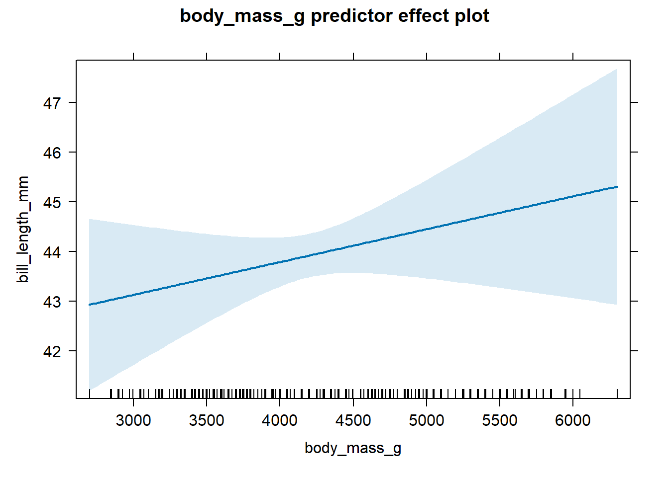
Figure 4.1: Effect plot for body mass based on the fitted model in Equation (4.8).
We see from Figure 4.1 that there is a
clear positive association between body_mass_g and bill_length_mm
after accounting for the flipper_length_mm variable. The shaded area
indicates the 95% confidence interval bands for the estimated mean
response. We do not discuss confidence interval bands here, except to
say that they provide a visual picture of the uncertainty of our
estimated mean (wider bands indicate greater uncertainty). Chapter
6 discusses confidence intervals for linear models in
some detail. The many tick marks along the the x-axis of the effect plot
indicate observed values of the x-axis variable.
We next create an effect plot for flipper_length_mm, which is shown in
Figure 4.2, using the code below.
There is a clear positive association between flipper_length_mm and
bill_length_mm after accounting for body_mass_g.
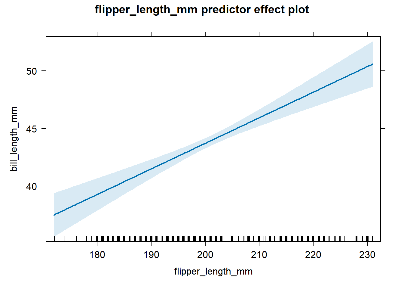
Figure 4.2: Effect plot for flipper length based on the fitted model in Equation (4.8).
Alternatively, we could use effects::allEffects to compute the
necessary effect plot information for all predictors simultaneously,
then use plot to create a display of the effect plots for all
predictors in one graphic. This approach is quicker, but the individual
effect plots can sometimes be too small for practical use. We
demonstrate this faster approach in the code below, which produces
Figure 4.3.
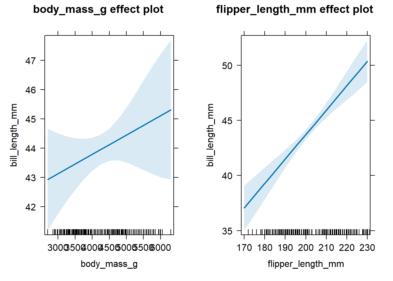
Figure 4.3: All effect plots for predictors of the fitted model in Equation (4.8).
4.3 Interpretation for categorical predictors
We now discuss the interpretation of regression coefficients in the context of a parallel lines and separate lines models.
4.3.1 Coefficient interpretation for parallel lines models
Consider a parallel lines model with numeric regressor \(X\) and categorical predictor \(C\) with levels \(L_1\), \(L_2\), and \(L_3\). Following the discussion in Section 3.8, predictor \(C\) must be transformed into two indicator variables, \(D_2\) and \(D_3\), for category levels \(L_2\) and \(L_3\), to be included in our linear model. \(L_1\) is the reference level. The parallel lines model is formulated as \[ E(Y \mid X, C) = \beta_{int} + \beta_{X} X + \beta_{L_2} D_2 + \beta_{L_3} D_3, \tag{4.9} \] where we replace the usual \(\beta_0\), \(\beta_1\), \(\beta_2\), and \(\beta_3\) with notation the indicates the regressor each coefficient is associated with.
When an observation has level \(L_1\) and \(X=0\), then the expected response is \[ \begin{aligned} E(Y|X = 0, C=L_1) &= \beta_{int} + \beta_X \cdot 0 + \beta_{L_2} \cdot 0 + \beta_{L_3} \cdot 0 \\ &= \beta_{int}. \end{aligned} \] Thus, \(\beta_{int}\) is the expected response for an observation with level \(L_1\) when \(X=0\).
When an observation has a fixed level \(L_j\) (it doesn’t matter which level) and \(X\) increases from \(x^*\) to \(x^*+1\), then the change in the expected response is \[ E(Y|X = x^* + 1, C=L_j) - E(Y|X = x^*, C=L_j)= \beta_X. \] Thus, \(\beta_X\) is the expected change in the response for an observation with fixed level \(L_j\) when \(X\) increases by 1 unit.
When an observation has level \(L_2\), the expected response is \[ \begin{aligned} E(Y\mid X = x^*, C=L_2) &= \beta_{int} + \beta_X x^* + \beta_{L_2} \cdot 1 + \beta_{L_3} \cdot 0 \\ &= \beta_{int} + \beta_X x^* + \beta_{L_2}. \end{aligned} \] Thus, \[ \begin{aligned} & E(Y\mid X=x^*, C=L_2) - E(Y\mid X=x^*, C=L_1) \\ &= (\beta_{int} + \beta_X x^* + \beta_{L_2}) - (\beta_{int} + \beta_X x^*) \\ &= \beta_{L_2}. \end{aligned} \] Thus, \(\beta_{L_2}\) is the expected change in the response for a fixed value of \(X\) when comparing on observation having level \(L_1\) to level \(L_2\) of predictor \(C\). More specifically, \(\beta_{L_2}\) indicates the distance between the estimated regression lines for observations having levels \(L_1\) and \(L_2\). A similar interpretation holds for \(\beta_{L_3}\) when comparing observations having level \(L_3\) to observations having level \(L_1\). \(L_1\) is known as as the reference level of \(C\) because we must refer to it to interpret our model with respect to other levels of \(C\).
To summarize the interpretation of the coefficients in parallel lines models like Equation (4.9), assuming categorical predictor \(C\) has \(K\) levels instead of 3:
- \(\beta_{int}\) represents the expected response for observations having the reference level when the numeric regressor \(X = 0\).
- \(\beta_X\) is the expected change in the response when \(X\) increases by 1 unit for a fixed level of \(C\).
- \(\beta_{L_j}\), for \(j=2,\ldots,K\), represents the expected change in the response when comparing observations having level \(L_1\) and \(L_j\) with \(X\) fixed at the same value.
In Section 3.9, we fit a parallel lines model to the
penguins data that used both body_mass_g and species to explain
the behavior of bill_length_mm. Letting \(D_C\) denote the indicator
variable for the Chinstrap level and \(D_G\) denote the indicator
variable for the Gentoo level, the fitted parallel lines model was
\[
\begin{aligned}
&\hat{E}(\mathtt{bill\_length\_mm} \mid \mathtt{body\_mass\_g}, \mathtt{species})\\
&= 24.92 + 0.004 \mathtt{body\_mass\_g} + 9.92 D_C + 3.56 D_G.
\end{aligned}
\]
In the context of this model:
- The expected bill length for an Adelie penguin with a body mass of 0 grams is 24.92 mm.
- If two penguins are of the same species, but one penguin has a body mass 1 gram larger, then the larger penguin is expected to have a bill length 0.004 mm longer than the smaller penguin.
- A Chinstrap penguin is expected to have a bill length 9.92 mm longer than an Adelie penguin, assuming their body mass is the same.
- A Gentoo penguin is expected to have a bill length 3.56 mm longer than an Adelie penguin, assuming their body mass is the same.
4.3.2 Effect plots for fitted models with non-interacting categorical predictors
How do we create an effect plot for a numeric focal predictor when a non-interacting categorical predictor is in the model (such as for the parallel lines model we have been discussing)? In short, we determine the fitted model equation as a function of the focal predictor for each level of the categorical predictor, and then compute the weighted average of the equation with the weights being proportional to the number of observations in each group.
Let’s construct an effect plot for the body_mass_g predictor in the
context of the penguins parallel lines model discussed in the previous
section. In Section 3.9, we determined that the
fitted parallel lines model simplified to the following equations
depending on the level of species:
\[
\begin{aligned}
&\hat{E}(\mathtt{bill\_length\_mm} \mid \mathtt{body\_mass\_g}, \mathtt{species}=\mathtt{Adelie}) \\
&= 24.92 + 0.004 \mathtt{body\_mass\_g} \\
&\hat{E}(\mathtt{bill\_length\_mm} \mid \mathtt{body\_mass\_g}, \mathtt{species}=\mathtt{Chinstrap}) \\
&= 34.84 + 0.004 \mathtt{body\_mass\_g} \\
&\hat{E}(\mathtt{bill\_length\_mm} \mid \mathtt{body\_mass\_g}, \mathtt{species}=\mathtt{Gentoo}) \\
&= 28.48 + 0.004 \mathtt{body\_mass\_g}.
\end{aligned}
\tag{4.10}
\]
We recreate the fitted model producing these equations in R using the
code below.
# refit the parallel lines model
lmodp <- lm(bill_length_mm ~ body_mass_g + species, data = penguins)
# double-check coefficients
coef(lmodp)
##      (Intercept)      body_mass_g speciesChinstrap
##     24.919470977      0.003748497      9.920884113
##    speciesGentoo
##      3.557977539
The code below determines the number of observations with each level of
species for the data used in the fitted model lmodp. We see that 151
Adelie, 68 Chinstrap, and 123 Gentoo penguins (342 total penguins) were
used to fit the model stored in lmodp.
The equation used to create the effect plot of body_mass_g is the
weighted average of the equations in Equation (4.10),
with weights proportional to the number of observational having each
level of the categorical predictor. Specifically,
\[
\begin{aligned}
& \hat{E}(\mathtt{bill\_length\_mm} \mid \mathtt{body\_mass\_g}, \mathtt{species}=\mathtt{typical}) \\
&= \frac{151}{342}(24.92 + 0.004 \mathtt{body\_mass\_g})\\
&\quad + \frac{68}{342}(34.84 + 0.004 \mathtt{body\_mass\_g})\\
&\quad + \frac{123}{342}(28.48 + 0.004 \mathtt{body\_mass\_g}) \\
&=28.17 + 0.004 \mathtt{body\_mass\_g}.
\end{aligned}
\]
The effect plot for body_mass_g for the fitted parallel lines model
is shown in Figure 4.4. The
association between bill_length_mm and body_mass_g is positive after
accounting for species.
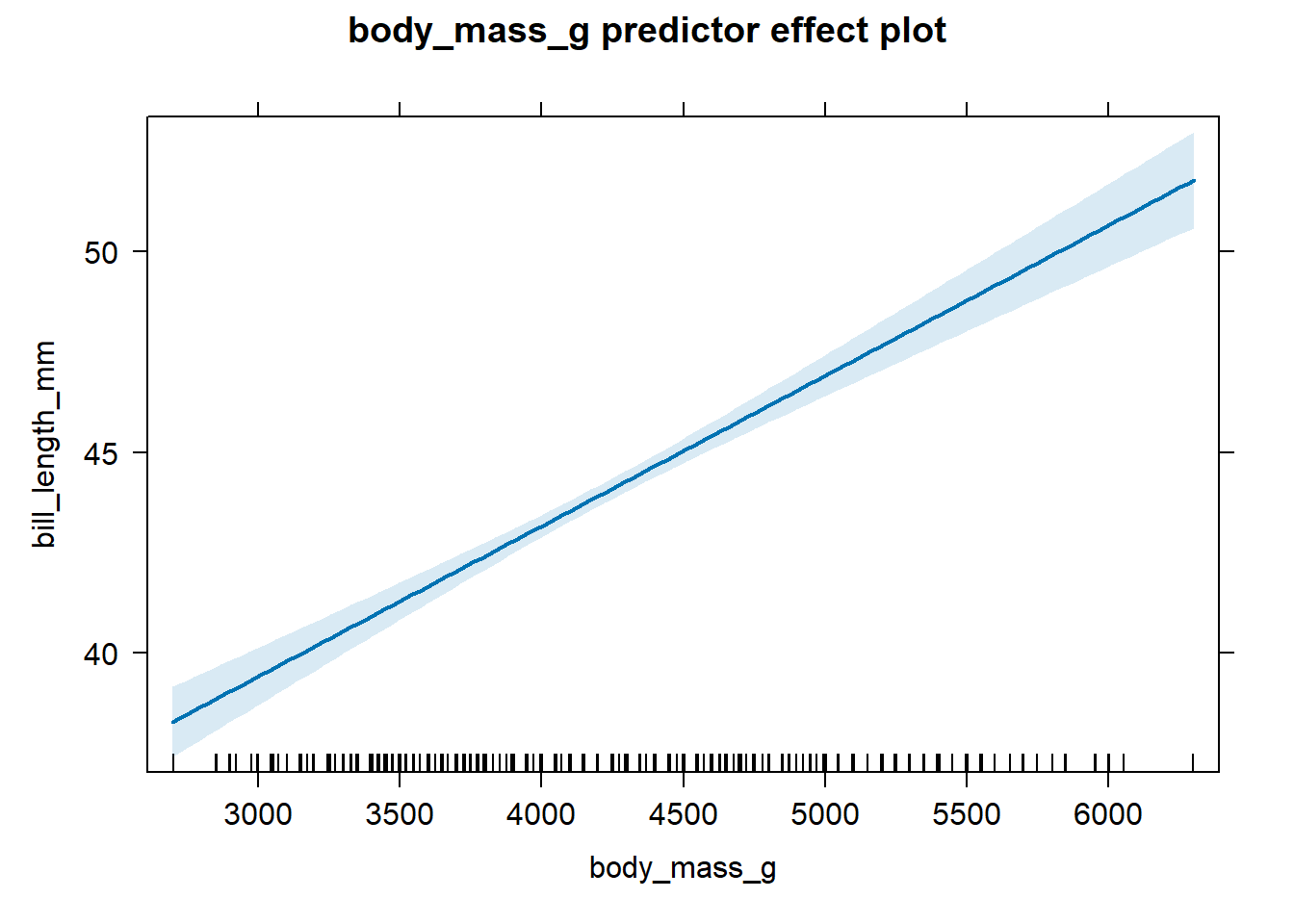
Figure 4.4: The effect plot of body_mass_g for the fitted parallel lines model.
An effect plot for a categorical predictor, assuming all other
predictors in the model are non-interacting numerical predictors (i.e.,
fixed group predictors), is a plot of the estimated mean response for
each level of the categorical variable when the fixed group group
predictors are held at their sample mean. The sample mean of the
body_mass_g values used to fit lmodp is 4201.75, as shown in the
code below.
# sample mean of body_mass_g variable used to fit lmodp
mean(lmodp$model$body_mass_g)
## [1] 4201.754
Using the first equation in Equation (4.10), the
estimated mean for the Adelie species when body_mass_g is fixed at
4201.75 is
\[
\begin{aligned}
&\hat{E}(\mathtt{bill\_length\_mm} \mid \mathtt{body\_mass\_g} = 4201.75, \mathtt{species}=\mathtt{Adelie}) \\
&= 24.92 + 0.004 \cdot 4201.75 \\
&= 40.67.
\end{aligned}
\]
Similarly,
\(\hat{E}(\mathtt{bill\_length\_mm} \mid \mathtt{body\_mass\_g} = 4201.75, \mathtt{species}=\mathtt{Chinstrap}) = 50.59\)
and
\(\hat{E}(\mathtt{bill\_length\_mm} \mid \mathtt{body\_mass\_g} = 4201.75, \mathtt{species}=\mathtt{Gentoo}) = 44.23\).
The code below produces the effect plot for species, which is shown in
Figure 4.5. We see that after accounting
for body_mass_g, the bill_length_mm tends to be largest for
Chinstrap penguins, second largest for Gentoo penguins, and smallest for
Adelie penguins. The confidence bands for the estimated mean response
are shown by the vertical bars.
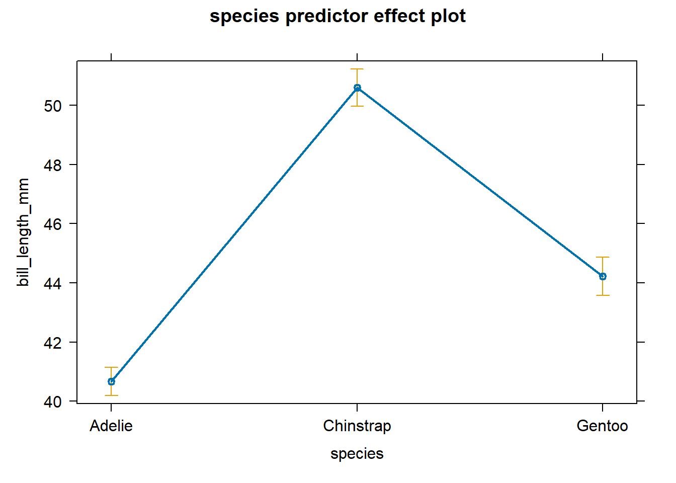
Figure 4.5: An effect plot for species after accounting for body_mass_g.
4.3.3 Coefficient interpretation for separate lines models
Consider a separate lines model with numeric regressor \(X\) and categorical predictor \(C\) with levels \(L_1\), \(L_2\), and \(L_3\). The predictor \(C\) will be transformed into two indicator variables, \(D_2\) and \(D_3\), for category levels \(L_2\) and \(L_3\), with \(L_1\) being the reference level. The separate lines model is formulated as \[ E(Y \mid X, C) = \beta_{int} + \beta_{X} X + \beta_{L_2} D_2 + \beta_{L_3} D_3 + \beta_{XL_2} XD_2+\beta_{XL_3}XD_3. \tag{4.11} \]
When an observation has level \(L_1\) and \(X=x^*\), then the expected response is \[ \begin{aligned} &E(Y\mid X = x^*, C=L_1) \\ &= \beta_{int} + \beta_X \cdot x^* + \beta_{L_2} \cdot 0 + \beta_{L_3} \cdot 0 + \beta_{X L_2} \cdot x^* \cdot 0 + \beta_{X L_3}\cdot x^* \cdot 0 \\ &= \beta_{int} + \beta_X x^*. \end{aligned} \tag{4.12} \]
Using Equation (4.12), we can verify that:
- \(\beta_{int} = E(Y\mid X = 0, C=L_1)\).
- \(\beta_{X} = E(Y\mid X = x^* + 1, C=L_1) - E(Y\mid X = x^*, C=L_1)\).
Similarly, when \(C=L_2\), \[ \begin{aligned} & E(Y|X = x^*, C=L_2) \\ &= \beta_{int} + \beta_X \cdot x^* + \beta_{L_2} \cdot 1 + \beta_{L_3} \cdot 0 + \beta_{X L_2} \cdot x^* \cdot 1 + \beta_{X L_3}\cdot x^* \cdot 0 \\ &= \beta_{int} + \beta_X x^* + \beta_{L_2} + \beta_{XL_2}x^*\\ &= (\beta_{int} + \beta_{L_2}) + (\beta_X + \beta_{XL_2})x^*. \end{aligned} \tag{4.13} \] Following this same pattern, when \(C=L_3\) we have \[ E(Y|X = x^*, C=L_3) = (\beta_{int} + \beta_{L_3}) + (\beta_X + \beta_{XL_3})x^*. \tag{4.14} \]
Using Equations (4.12), (4.13), and (4.14), we can verify that for \(j=2,3\), \[ \beta_{L_j}= E(Y\mid X = 0, C=L_j) - E(Y\mid X = 0, C=L_1), \] and \[ \begin{aligned} & \beta_{XL_j} \\ &= [E(Y\mid X = x^*+1, C=L_j) - E(Y\mid X = x^*, C=L_j)]\\ &\quad-[E(Y\mid X = x^*+1, C=L_1) - E(Y\mid X = x^*, C=L_1)]. \end{aligned} \]
To summarize the interpretation of the coefficients in separate lines models like Equation (4.11), assuming categorical predictor \(C\) has \(K\) levels instead of 3:
- \(\beta_{int}\) represents the expected response for observations having the reference level when the numeric regressor \(X = 0\).
- \(\beta_{L_j}\), for \(j=2,\ldots,K\), represents the expected change in the response when comparing observations having level \(L_1\) and \(L_j\) with \(X=0\).
- \(\beta_X\) represents the expected change in the response when \(X\) increases by 1 unit for observations having the reference level.
- \(\beta_{X L_j}\), for \(j=2,\ldots,K\), represents the difference in the expected response between observations having the reference level in comparison to level \(L_j\) when \(X\) increases by 1 unit. More simply, these terms represent the difference in the rate of change for observations having level \(L_j\) compared to the reference level.
We illustrate these interpretation using the separate lines model to the
penguins data in Section 3.9. The fitted
separate lines model was
\[
\begin{aligned}
&\hat{E}(\mathtt{bill\_length\_mm} \mid \mathtt{body\_mass\_g}, \mathtt{species}) \\
&= 26.99 + 0.003 \mathtt{body\_mass\_g} + 5.18 D_C - 0.25 D_G \\
&\quad + 0.001 D_C \mathtt{body\_mass\_g} + 0.0009 D_G \mathtt{body\_mass\_g}.
\end{aligned}
\tag{4.15}
\]
In the context of this model:
- The expected bill length for an Adelie penguin with a body mass of 0 grams is 26.99 mm.
- If an Adelie penguin has a body mass 1 gram larger than another Adelie penguin, then the larger penguin is expected to have a bill length 0.003 mm longer than the smaller penguin.
- A Chinstrap penguin is expected to have a bill length 5.18 mm longer than an Adelie penguin when both have a body mass of 0 grams.
- A Gentoo penguin is expected to have a bill length 0.25 mm shorter than an Adelie penguin when both have a body mass of 0 grams.
- For each 1 gram increase in body mass, we expect the change in bill length by Chinstrap penguins to be 0.001 mm larger than the corresponding change in bill length by Adelie penguins.
- For each 1 gram increase in body mass, we expect the change in bill length by Gentoo penguins to be 0.0009 mm larger than the corresponding change in bill length by Adelie penguins.
4.3.4 Effect plots for interacting categorical predictors
We now discuss construction of effect plots for a separate lines model, which has an interaction between a categorical and numeric predictor. In additional to the focal and fixed group predictors we have previously discussed, Fox and Weisberg (2020) also discuss predictors in the conditioning group, which is the set of predictors that interact with the focal predictor.
When some predictors interact with the focal predictor, the effect plot of the focal predictor is a plot of the estimated mean response when the fixed group predictors are held at their typical values and the conditioning group predictors vary over different combinations of discrete values. The process of determining the estimated mean response as function of the focal predictor is similar to before, but there are more predictor values on which to condition. By default, to compute the estimated mean response as a function of the focal predictor, we:
- Hold the numeric fixed group predictors at their sample means.
- Average the estimated mean response equation across the different levels of a fixed group categorical predictor, with weights equal to the number of observations with each level.
- Compute the estimated mean response function for 5 discrete values of numeric predictors in the conditioning group.
- Compute the estimated mean response function for different levels of a categorical predictor in the conditioning group.
We provide examples of the effect plots for the body_mass_g and
species predictors for the separate lines model fit to the penguins
data and given in Equation (4.15). We first run the
code below to fit the separate lines model previously fit in Section
3.9.
# fit separate lines model
lmods <- lm(bill_length_mm ~ body_mass_g + species + body_mass_g:species,
            data = penguins)
# extract estimated coefficients
coef(lmods)
##                  (Intercept)                  body_mass_g
##                26.9941391367                 0.0031878758
##             speciesChinstrap                speciesGentoo
##                 5.1800537287                -0.2545906615
## body_mass_g:speciesChinstrap    body_mass_g:speciesGentoo
##                 0.0012748183                 0.0009029956
We previously determined in Section 3.9 that the model simplifies depending on the level of species. Specifically, we have that \[ \begin{aligned} &\hat{E}(\mathtt{bill\_length\_mm} \mid \mathtt{body\_mass\_g}, \mathtt{species}=\mathtt{Adelie}) \\ &= 26.99 + 0.003 \mathtt{body\_mass\_g},\\ &\hat{E}(\mathtt{bill\_length\_mm} \mid \mathtt{body\_mass\_g}, \mathtt{species}=\mathtt{Chinstrap}) \\ &= 31.17 + 0.004 \mathtt{body\_mass\_g},\\ &\hat{E}(\mathtt{bill\_length\_mm} \mid \mathtt{body\_mass\_g}, \mathtt{species}=\mathtt{Gentoo}) \\ &= 26.74 + 0.004 \mathtt{body\_mass\_g}. \end{aligned} \tag{4.16} \]
The effect plot of body_mass_g for the separate lines model will be a
plot of each equation given in Equation
(4.16). Figure
4.6 displays this effect plot, which
was created using the code below. We use the axes argument to rotate
the x-axis labels (otherwise the text overlaps) and the lines
argument to display all three lines in one graphic instead of a
separate panel for each level of species. We notice Chinstrap penguins
tend to have the largest bill lengths for a given value of body mass and
the bill lengths increase more quickly as a function of body mass then
for the Adelie and Gentoo penguins. Similarly, the Adelie penguins tend
to have the smallest bill length for a fixed value of body mass and the
bill length tends to increase more slowly as body mass increases
compared to the other two types of penguins.
# effect plot of body mass for separate lines model
# axes ... rotates the x-axis labels 90 degrees
# lines ... plots the effect of body mass in one graphic
plot(predictorEffect("body_mass_g", lmods),
     axes = list(x = list(rotate = 90)),
     lines = list(multiline = TRUE))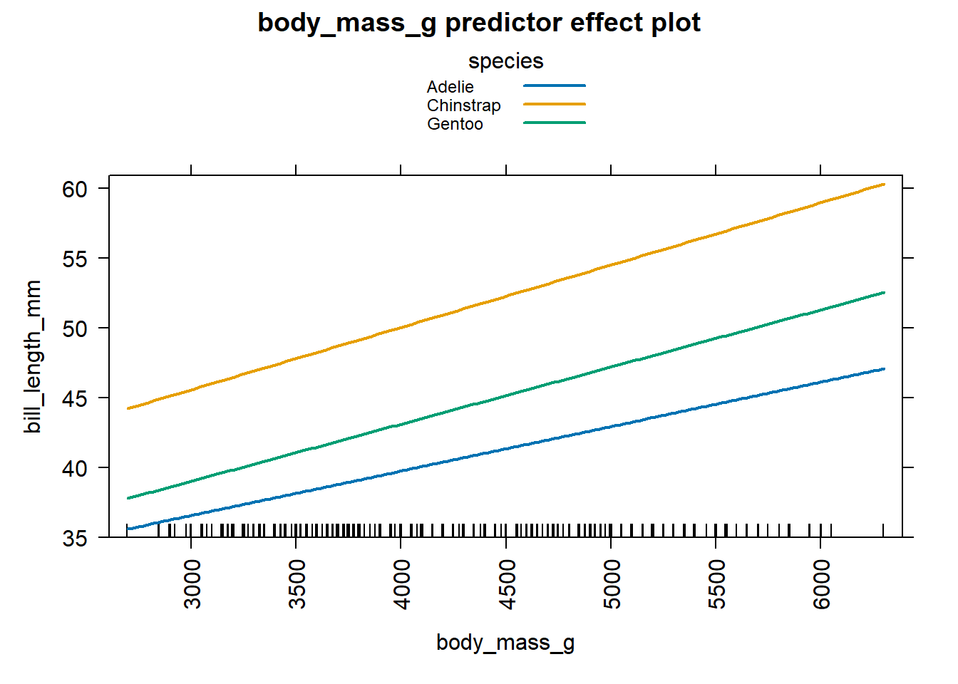
Figure 4.6: Effect plot for body mass based on the equations in Equation (4.16).
The effect plot of species for the separate lines model will be a plot
of the estimated mean response in Equation
(4.16) for each level of
species when varying body_mass_g over 5 discrete values. Figure
4.7 displays this effect plot, which
was created using the code below. By specifying
lines = list(multiline = TRUE), the estimated mean responses for each
level of species are connected for each discrete value of
body_mass_g. Figure 4.7 allows us to
determine the effect of species on bill_length_mm when we vary
body_mass_g over 5 discrete values. When varying body_mass_g across
the values 2700, 3600, 4500, 5300, and 6300 g, we see greater changes in
the estimated mean of bill_lengh_mm for Chinstrap penguins in
comparison to Adelie and Gentoo penguins.
# effect plot of body mass for separate lines model
# axes ... rotates the x-axis labels 90 degrees
# lines ... plots the effect of species in one graphic
plot(predictorEffect("species", lmods),
     axes = list(x = list(rotate = 90)),
     lines=list(multiline = FALSE))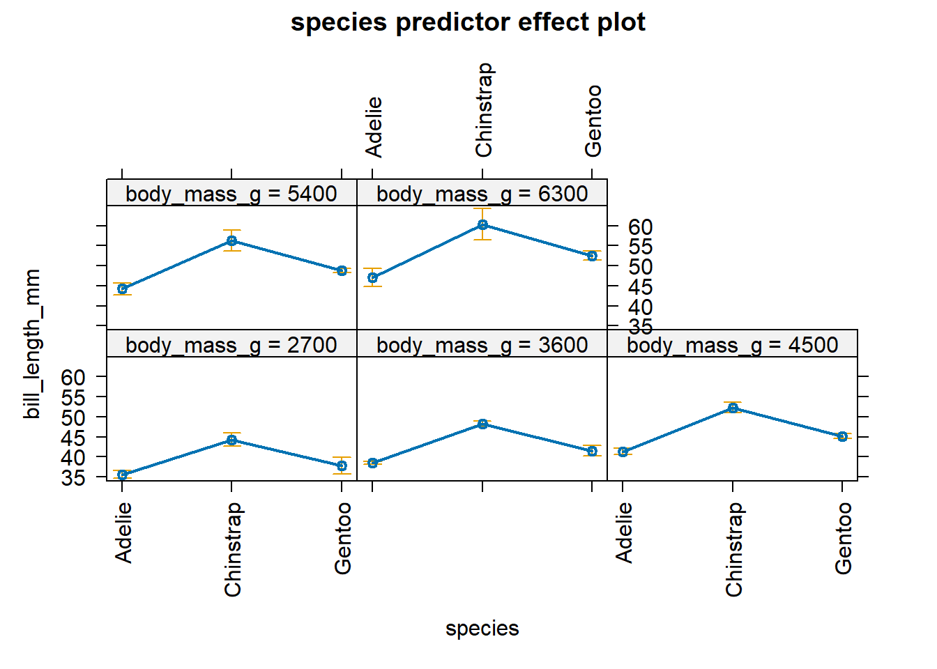
Figure 4.7: Effect plot for species based on the equations in Equation (4.16).
We refer the reader to the “Predictor effects gallery” vignette in the
effects package (run
vignette("predictor-effects-gallery", package = "effects") in the
Console) for more details about how to construct effect plots in
different settings.
4.4 Added-variable and leverage plots
In this section, we will use visual displays to assess the impact of a predictor after accounting for the impact of other preditors already in the model.
An added-variable plot or partial regression plot displays the marginal effect of a regressor on the response after accounting for the other regressors in the model (Mosteller and Tukey 1977). While an effect plot is a plot of the estimated mean relationship between the response and a focal predictor while holding the model’s predictors at typical values, the added-variable plot is a plot of two sets of residuals against one other.
We create an added-variable plot for regressor \(X_j\) in the following way:
- Compute the residuals of the model regressing the response \(Y\) on all regressors except \(X_j\). We denote these residuals \(\hat{\boldsymbol{\epsilon}}(Y\mid \mathbb{X}_{-j})\). These residuals represent the part of the response variable not explained by the regressors in \(\mathbb{X}_{-j}\).
- Compute the residuals of the model regressing the regressor \(X_j\) on all regressors except \(X_j\). We denote these residuals \(\hat{\boldsymbol{\epsilon}}(X_j \mid \mathbb{X}_{-j})\). These residuals represent the part of the \(X_j\) not explained by the regressors in \(\mathbb{X}_{-j}\). Alternatively, these residuals represent the amount of additional information \(X_j\) provides after accounting for the regressors in \(\mathbb{X}_{-j}\).
- The added-variable plot for \(X_j\) is a plot of \(\hat{\boldsymbol{\epsilon}}(Y\mid \mathbb{X}_{-j})\) on the y-axis and \(\hat{\boldsymbol{\epsilon}}(X_j \mid \mathbb{X}_{-j})\) on the x-axis.
Added-variable plots allow us to visualize the impact a regressor has when added to an existing regression model. We can use the added-variable plot for \(X_j\) to visually estimate the partial slope \(\hat{\beta}_{j}\) (Sheather 2009). In fact, the simple linear regression line that minimizes the RSS for the added-variable plot of \(X_j\) will have slope \(\hat{\beta}_j\).
We can use an added-variable plot in several ways:
- To assess the marginal relationship between \(X_j\) and \(Y\) after accounting for all of the other variables in the model.
- To assess the strength of this marginal relationship.
- To identify deficiencies in our fitted model.
- To identify outliers and observations influential in determining the estimated partial slope.
We focus on points 1 and 2 above, as they are directly related to interpreting our fitted model. We discuss points 3 and 4 in the context of diagnostics for assessing the appropriateness of our model.
In regards to point 1 and 2:
- If the added-variable plot for \(X_j\) is essentially a scatter of points with slope zero, then \(X_j\) can do little to explain \(Y\) after accounting for the other regressors. There is little to gain in adding \(X_j\) as an additional regressor to the model regressing \(Y\) on \(\mathbb{X}_{-j}\). Figure 4.8 (a) provides an example of this situation.
- If the points in an added-variable plot for \(X_j\) have a linear relationship, then adding \(X_j\) to the model regressing \(Y\) on \(\mathbb{X}_{-j}\) is expected to improve our model’s ability to predict the behavior of \(Y\). The stronger the linear relationship of the points in the added-variable plot, the more important this variable tends to be in our model. Figure 4.8 (b) demonstrates this scenario.
In regard to point 3, if the points in an added-variable plot for \(X_j\) are curved or non-linear, it indicates that that there is a deficiency in the fitted model (likely because we need to include one or more additional regressors to the model). Figure 4.8 (c) provides an example of this situation.
In relation to point 4, if certain points in the added-variable plot seem to “pull” the fitted line toward themselves so that the line doesn’t fit the bulk of the data, that indicates the presence of influential observations that are substantially influencing the fit of the model to the data. Figure 4.8 (d) provides an example of this situation.
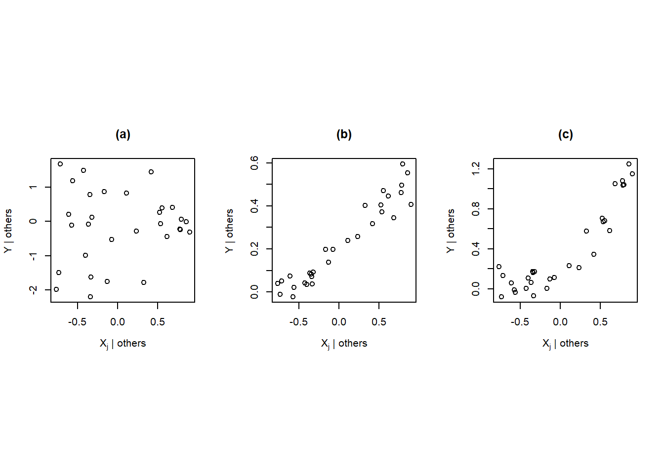
Figure 4.8: Examples of added-variable plots
The car package (Fox, Weisberg, and Price 2024) provides the avPlot and avPlots
functions for creating added-variable plots. The avPlot function will
produce an added-variable plot for a single regressor while the
avPlots function will produce added-variable plots for one or more
regressors.
The main arguments to the avPlot function are:
model: the fittedlm(orglm) object.variable: the regressor for which to create an added-variable plot.id: a logical value indicating whether unusual observations should be identified. By default, the value isTRUE, which means the 2 points with the largest residuals and the 2 points with the largest partial leverage are identified, though this can be customized.
The avPlots function replaces the variable argument with the terms
argument. The terms argument should be a one-sided formula to indicate
the regressors for which we want to construct added-variable plots (one
plot for each term). By default, an added-variable plot is created for
each regressor. Run car::avPlot in the Console for information about
about the arguments and details of the avPlot and avPlots functions.
We now create and interpret added-variable plots for the model
regressing bill_length_mm on body_mass_g and flipper_length_mm,
which was previously assigned the name mlmod. We first load the
car package and then use the avPlots function to construct
added-variable plots for body_mass_g and flipper_length_mm. Figure
4.9 displays the added-variable plots for
body_mass_g and flipper_length_mm. The blue line is the simple
linear regression model that minimizes the RSS of the points. The
added-variable plot for body_mass_g exhibits a weak positive linear
relationship between the points. After using the flipper_length_mm
variable to explain the behavior of bill_length_mm, body_mass_g
likely has some additional explanatory power, but it doesn’t explain a
lot of additional response variation. The added-variable plot for
flipper_length_mm exhibits a slightly stronger positive linear
relationship. The flipper_length_mm variable seems to have some
additional explanatory power when added to the model regressing
bill_length_mm on body_mass_g.
library(car)
##
## Attaching package: 'car'
## The following object is masked from 'package:dplyr':
##
##     recode
## The following object is masked from 'package:purrr':
##
##     some
# create added-variable plots for all regressors in mlmod
avPlots(mlmod)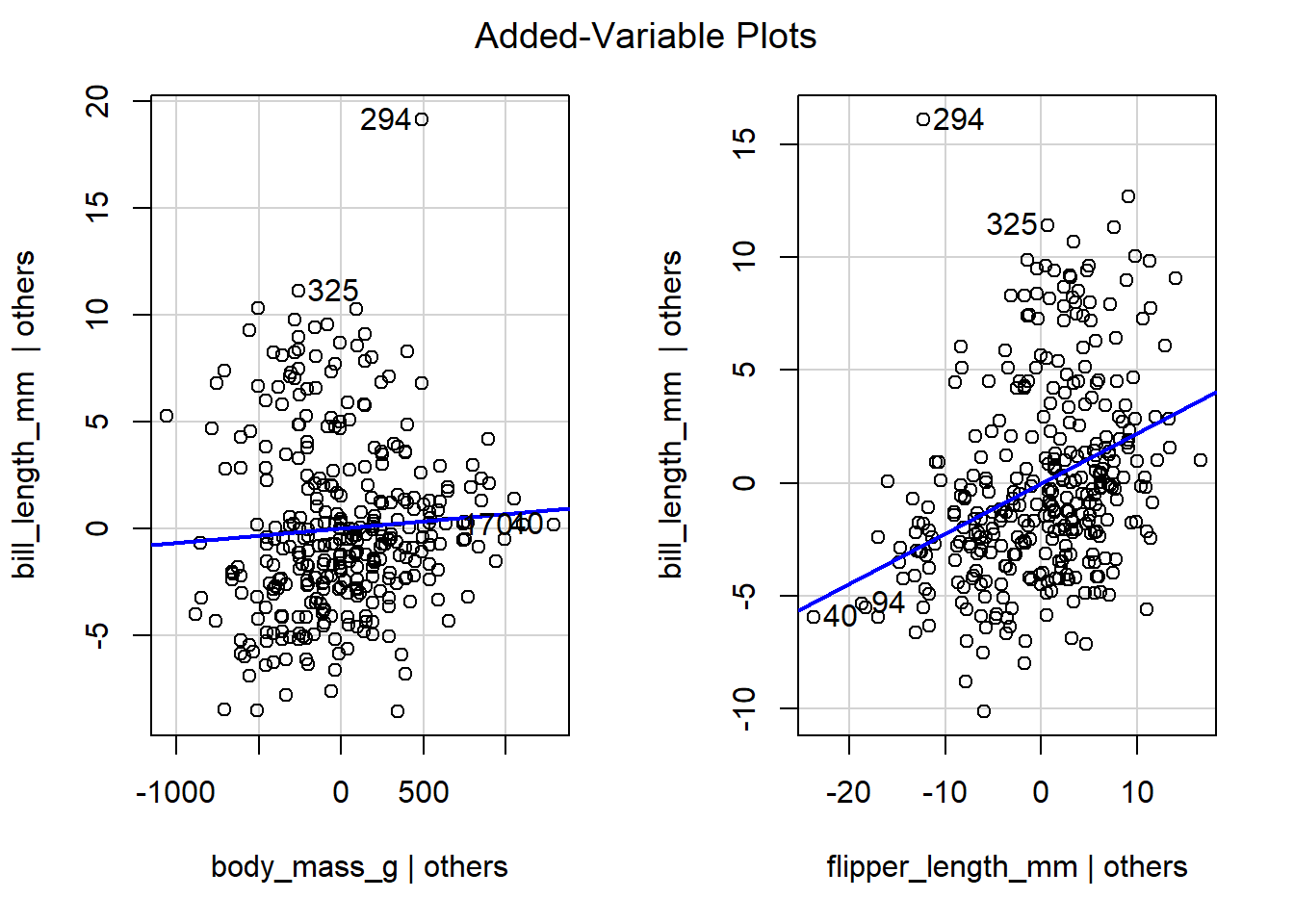
Figure 4.9: The added-variable plots of all regressors for the model regressing bill_length_mm on body_mass_g and flipper_length_mm.
The added-variable plots of fitted models with categorical predictors
often show “clusters” of points related to the categorical predictors.
These clusters aren’t anything to worry about unless the overall pattern
of the points is non-linear. We use the code below to create the
added-variable plots for all regressors in the parallel lines model
previously fit to the penguins data. The fitted model was
\[
\begin{aligned}
&\hat{E}(\mathtt{bill\_length\_mm} \mid \mathtt{body\_mass\_g}, \mathtt{species})\\
&= 24.92 + 0.004 \mathtt{body\_mass\_g} + 9.92 D_C + 3.56 D_G,
\end{aligned}
\]
where \(D_C\) and \(D_G\) are indicator variables for the Chinstrap and
Gentoo penguin species (Adelie penguins are the reference species).
Figure 4.10 displays the added-variable plots for
the body_mass_g regressor and the indicator variables for Chinstrap
and Gentoo penguins. The added-variable plot for body_mass_g has a
moderately strong linear relationship, so adding body_mass_g to the
model regressing bill_length_mm on species seems to be beneficial.
The other two variable plots also show a linear relationship. Clustering
patterns are apparent in the added-variable plot for the Chinstrap
penguins indicator variable (speciesChinstrap) but not for the Gentoo
penguins indicator variable.
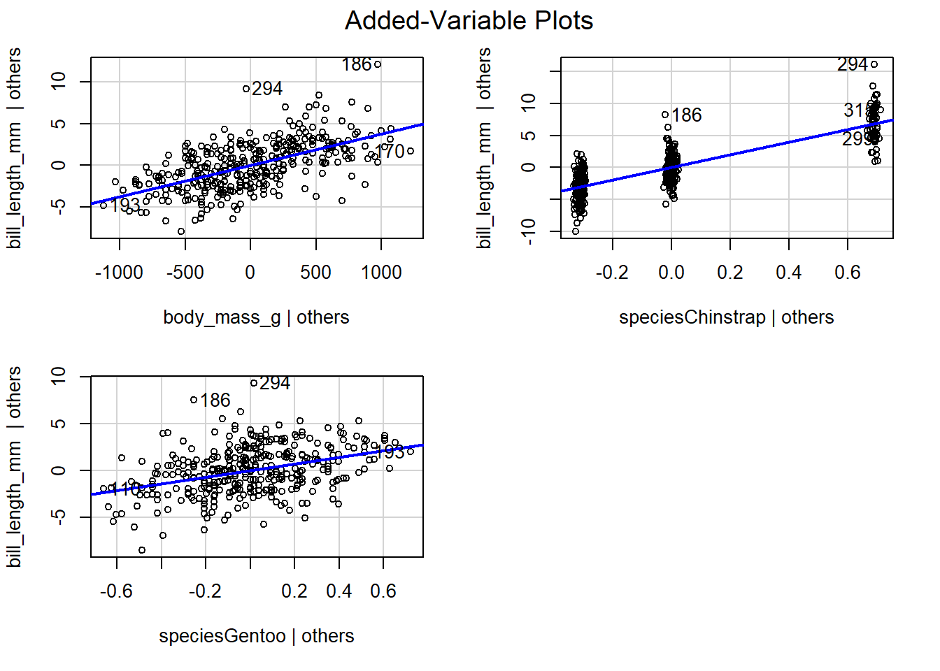
Figure 4.10: The added-variable plots for all regressors in the parallel lines model fit to the penguins data.
A challenge in interpreting the added-variable plots of indicator variable regressors is that it often doesn’t make sense to talk about the effect of adding a single regressor when all of the other regressors are in the model. Specifically, we either add the categorical predictor to our regression model or we do not. When we add a categorical predictor to our model, we simultaneously add \(K-1\) indicator variables as regressors; we do not add the indicator variables one-at-a-time. In general, we refer to regressors with this behavior as “multiple degrees-of-freedom terms”. A categorical variable with 3 or more levels is the most basic of multiple degrees-of-freedom term, but we can also consider regressors related to the interaction between two or more predictors, polynomial regressors, etc.
A leverage plot is an extension of the added-variable plot that
allows us to visualize the impact of multiple degrees-of-freedom terms.
Sall (1990) originally proposed leverage plots to visualize
hypothesis tests of linear hypotheses. The interpretation of leverage
plots is similar to the interpretation of added-variable plots, though
we refer to “predictors” or “terms” instead regressors (which may be
combined into one plot). The leveragePlot and leveragePlots
functions in the car package produce single or multiple leverage
plots, respectively, with arguments similar to the avPlot and
avPlots functions.
We use the code below to create Figure 4.11,
which displays leverage plots for the body_mass_g and species
predictors of the parallel lines model previously fit to the penguins
data. The leverage plot for body_mass_g has a moderate linear
relationship, so we expect body_mass_g to have moderate value in
explaining the behavior of bill_length_mm after accounting for
species. Similarly, the points in the leverage plot for species have
a moderately strong linear relationship, so we expect species to have
moderate value in explaining the behavior of bill_length_mm after
accounting for body_mass_g.
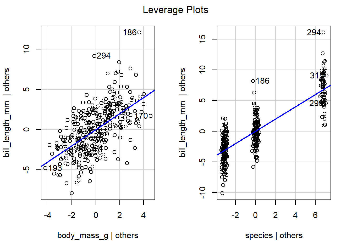
Figure 4.11: Leverage plots for the predictors in the parallel lines model fit to the penguins data.
We next examine the leverage plot for the separate lines model fit to
the penguins data. The fitted separate lines model is
\[
\begin{aligned}
&\hat{E}(\mathtt{bill\_length\_mm} \mid \mathtt{body\_mass\_g}, \mathtt{species}) \\
&= 26.99 + 0.003 \mathtt{body\_mass\_g} + 5.18 D_C - 0.25 D_G \\
&\quad + 0.001 D_C \mathtt{body\_mass\_g} + 0.0009 D_G \mathtt{body\_mass\_g},
\end{aligned}
\]
which has 6 estimated coefficients. However, the fitted model has only
3 non-intercept terms. Recall the formula we fit for the separate lines
model:
# function call for separate lines model
lm(formula = bill_length_mm ~ body_mass_g + species + body_mass_g:species,
   data = penguins)
Thus, we have terms for body_mass_g, species, and the interaction
term body_mass_g:species.
We use the code below to create the leverage plots shown in Figure
4.12. The leverage plot for body_mass_g has a
moderate linear relationship, so we expect body_mass_g to have
moderate additional value in explaining the behavior of bill_length_mm
after accounting for species and the interaction term
body_mass_g:species. It is unlikely we would include the
body_mass_g:species term in our model prior to including body_mass_g
, so philosophically, this plot provides little useful information.
Similarly, interpreting the leverage plot for species has limited
utility because the leverage plot includes the influence of the
interaction term body_mass_g:species. We are unlikely to fit a model
that includes the interaction term without also including the species
term directly. Instead it makes more sense to judge the utility of
adding species to the model regressing bill_length_mm on
body_mass_g alone, which we already considered in Figure
4.11. Examining the leverage plot for the
interaction term body_mass_g:species , we see the points have only a
weak linear relationship. Thus, we expect limited utility in adding the
interaction term body_mass_g:species to the parallel lines regression
model that regresses bill_length_mm on body_mass_g and species.
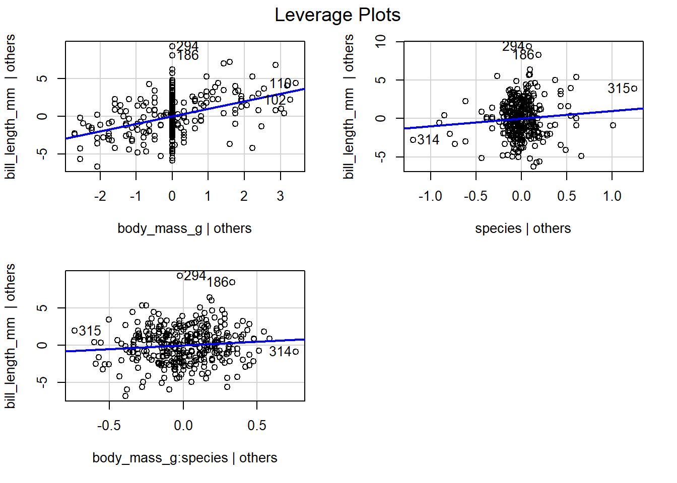
Figure 4.12: Leverage plots for the terms in the separate lines model fit to the penguins data.
4.5 Going deeper
4.5.1 Orthogonality
Let \[ \mathbf{X}_{[j]}=[x_{1,j},\ldots,x_{n,j}] \] denote the \(n\times 1\) column vector of observed values for column \(j\) of \(\mathbf{X}\). (We can’t use the notation \(\mathbf{x}_j\) because that is the \(p\times 1\) vector of regressor values for the \(j\)th observation).
Regressors \(\mathbf{X}_{[j]}\) and \(\mathbf{X}_{[k]}\) are orthogonal if \(\mathbf{X}_{[j]}^T \mathbf{X}_{[k]}=0\).
Let \(\boldsymbol{1}_{n\times1}\) denote an \(n\times 1\) column vector of 1s. The definition of orthogonal vectors above implies that \(\mathbf{X}_{[j]}\) is orthogonal to \(\boldsymbol{1}_{n\times1}\) if \[ \mathbf{X}_{[j]}^T \boldsymbol{1}_{n\times1} = \sum_{i=1}^n x_{i,j} = 0, \] i.e., if the values in \(\mathbf{X}_{[j]}\) sum to zero.
Let \(\bar{x}_j = \frac{1}{n}\sum_{i=1}^n x_{i,j}\) denote the sample mean of \(\mathbf{X}_{[j]}\) and \(\bar{\mathbf{x}}_j = \bar{x}_j \boldsymbol{1}_{n\times 1}\) denote the column vector that repeats \(\bar{x}_j\) \(n\) times.
Centering \(\mathbf{X}_{[j]}\) involves subtracting the sample mean of \(\mathbf{X}_{[j]}\) from \(\mathbf{X}_{[j]}\), i.e., \(\mathbf{X}_{[j]} - \bar{\mathbf{x}}_j\).
Regressors \(\mathbf{X}_{[j]}\) and \(\mathbf{X}_{[k]}\) are uncorrelated if they are orthogonal after being centered, i.e., if \[ (\mathbf{X}_{[j]} - \bar{\mathbf{x}}_j)^T (\mathbf{X}_{[k]} - \bar{\mathbf{x}}_k)=0. \] Note that the sample covariance between vectors \(\mathbf{X}_{[j]}\) and \(\mathbf{X}_{[k]}\) is \[ \begin{aligned} \widehat{\mathrm{cov}}(\mathbf{X}_{[j]}, \mathbf{X}_{[k]}) &= \frac{1}{n-1}\sum_{i=1}^n (x_{i,j} - \bar{x}_j)(x_{i,k} - \bar{x}_k) \\ &= \frac{1}{n-1}(\mathbf{X}_{[j]} - \bar{\mathbf{x}}_j)^T (\mathbf{X}_{[k]} - \bar{\mathbf{x}}_k). \end{aligned} \] Thus, two centered regressors are orthogonal if their covariance is zero.
It is a desirable to have orthogonal regressors in our fitted model because they simplify estimating the relationship between the regressors and the response. Specifically:
If a regressor is orthogonal to all other regressors (and the column of 1s) in a model, adding or removing the orthogonal regressor from our model will not impact the estimated regression coefficients of the other regressors.
Since most linear regression models include an intercept, we should assess whether our regressors are orthogonal to other regressors and the column of 1s.
We consider a simple example with \(n=5\) observations to demonstrate how orthogonality of regressors impacts the estimated regression coefficients.
In the code below:
yis a vector of response values.X1is a column vector of regressor values.X2is a column vector of regressor values chosen to be orthogonal toX1.
y <- c(1, 4, 6, 8, 9)       # create an arbitrary response vector
X1 <- c(7, 5, 5, 7, 7)      # create regressor 1
X2 <- c(-1, 2, -3, 1, 5/7)  # create regressor 2 to be orthogonal to X1
Note that the crossprod function computes the cross product of two vectors or matrices, so that crossprod(A, B) computes \(\mathbf{A}^T B\), where the vectors or matrices must have the correct dimension for the multiplication to be performed.
The regressor vectors X1 and X2 are orthogonal since their cross product \(\mathbf{X}_{[1]}^T \mathbf{X}_{[2]}\) (in R, crossprod(X1, X2)) equals zero, as shown in the code below.
In the code below, we regress y on X1 without an intercept (lmod1). The estimated coefficient for X1 is \(\hat{\beta}_1=0.893\).
Next, we then regress y on X1 and X2 without an intercept (lmod2). The estimated coefficients for X1 and X2 are \(\hat{\beta}_1=0.893\) and \(\hat{\beta}_2=0.221\), respectively. Because X1 and X2 are orthogonal (and because there are no other regressors to consider in the model), the estimated coefficient for X1 stays the
same in both models.
# y regressed on X1 and X2 without an intercept
lmod2 <- lm(y ~ X1 + X2 - 1)
coef(lmod2)
##        X1        X2
## 0.8934010 0.2210526
The previous models (lmod1 and lmod2) neglect an important characteristic of a typical linear model: we usually include an intercept coefficient (a columns of 1s as a regressor) in our model. If the regressors are not orthogonal to the column of 1s in our \(\mathbf{X}\) matrix, then the coefficients for the other regressors in
the model will change when the regressors are added or removed from the model because they are not orthogonal to the column of 1s.
We create a vector ones that is simply a column of 1s.
Neither X1 nor X2 is orthogonal with the column of ones. We compute the cross product between ones and the two regressors X1 and X2. Since the cross products are not zero, X1 and X2 are not orthogonal to the
column of ones.
crossprod(ones, X1) # not zero, so not orthogonal
##      [,1]
## [1,]   31
crossprod(ones, X2) # not zero, so not orthogonal
##            [,1]
## [1,] -0.2857143
We create lmod3 by adding adding a column of ones to lmod2 (i.e.,
we include the intercept in the model). The the coefficients for both
X1 and X2 change when going from lmod2 to lmod3 because these
regressors are not orthogonal to the column of 1s. Comparing the
coefficients lmod2 above and lmod3, \(\hat{\beta}_1\) changes from
\(0.893\) to \(0.397\) and \(\hat{\beta}_2\) changes from \(0.221\) to \(0.279\).
coef(lmod2) # coefficients for lmod2
##        X1        X2
## 0.8934010 0.2210526
# y regressed on X1 and X2 with an intercept
lmod3 <- lm(y ~ X1 + X2)
coef(lmod3) # coefficients for lmod3
## (Intercept)          X1          X2
##   3.1547101   0.3969746   0.2791657
For orthogonality of our regressors to be most impactful, the model’s
regressors should be orthogonal to each other and the column of 1s. In
that context, adding or removing any of the regressors doesn’t impact
the estimated coefficients of the other regressors. In the code below,
we define centered regressors X3 and X4 to be uncorrelated, i.e.,
X3 and X4 have sample mean zero and are orthogonal to each other.
X3 <-  c(0, -1, 1, 0, 0) # sample mean is zero
X4 <- c(0, 0, 0, 1, -1)  # sample mean is zero
cov(X3, X4)              # 0, so X3 and X4 are uncorrelated and orthogonal
## [1] 0
If we fit linear regression models with any combination of ones, X3,
or X4 as regressors, the associated regression coefficients will not
change. To demonstrate this, we consider all possible combinations of
the three variables in the models below. We do not run the code to save
space, but we summarize the results below.
coef(lm(y ~ 1))           # only column of 1s
coef(lm(y ~ X3 - 1))      # only X3
coef(lm(y ~ X4 - 1))      # only X4
coef(lm(y ~ X3))          # 1s and X3
coef(lm(y ~ X4))          # 1s and X4
coef(lm(y ~ X3 + X4 - 1)) # X3 and X4
coef(lm(y ~ X3 + X4))     # 1s, X3, and X4
We simply note that in each of the previous models, because all of the regressors (and the column of 1s) are orthogonal to each other, adding or removing any regressor doesn’t impact the estimated coefficients for the other regressors in the model. Thus, the estimated coefficients were \(\hat{\beta}_{0}=5.6\), \(\hat{\beta}_{3}=1.0\), \(\hat{\beta}_{4}=-0.5\) when the relevant regressor was included in the model.
The easiest way to determine which vectors are orthogonal to each other
and the intercept is to compute the cross product of the \(\mathbf{X}\)
matrix for the largest set of regressors we are considering. Consider
the matrix of cross products for the columns of 1s, X1, X2, X3, and
X4.
crossprod(model.matrix(~ X1 + X2 + X3 + X4))
##             (Intercept)  X1         X2 X3        X4
## (Intercept)   5.0000000  31 -0.2857143  0 0.0000000
## X1           31.0000000 197  0.0000000  0 0.0000000
## X2           -0.2857143   0 15.5102041 -5 0.2857143
## X3            0.0000000   0 -5.0000000  2 0.0000000
## X4            0.0000000   0  0.2857143  0 2.0000000
Consider the sequence of models below.
The model with only an intercept has an estimated coefficient of
\(\hat{\beta}_{0}=5.6\). If we add the X1 to the model with an
intercept, then the intercept coefficient changes because the column of 1s isn’t orthogonal to X1.
If we add X2 to lmod4, we might think that only \(\hat{\beta}_{0}\)
will change because X1 and X2 are orthogonal to each other. However,
because X2 is not orthogonal to all of the other regressors in the
model (X1 and the column of 1s), both \(\hat{\beta}_{0}\) and
\(\hat{\beta}_1\) will change. The easiest way to realize this is to look
at lmod2 above with only X1 and X2. When we add the column of 1s
to lmod2, both \(\hat{\beta}_1\) and \(\hat{\beta}_2\) will change because
neither regressor is orthogonal to the column of 1s needed to include
the intercept term.
However, note that X3 is orthogonal to the column of 1s and X1.
Thus, if we add X3 to lmod4, which includes both a column of 1s and
X1, X3 will not change the estimated coefficients for the intercept
or X1.
Additionally, since X4 is orthogonal to the column of 1s, X1, and
X3, adding X4 to the previous model will not change the estimated
coefficients for any of the other variables already in the model.
Lastly, if we can partition our \(\mathbf{X}\) matrix such that \(\mathbf{X}^T \mathbf{X}\) is a block diagonal matrix, then none of the blocks of variables will affect the estimated coefficients of the other variables.
Define a new regressor X5 below.
X5 is orthogonal to the column of
1s and X1, but not X4, as evidenced in the code below.
# note block of 0s
crossprod(cbind(ones, X1, X4, X5))
##      ones  X1 X4 X5
## ones    5  31  0  0
## X1     31 197  0  0
## X4      0   0  2 -1
## X5      0   0 -1  2
Note the block of zeros in the lower left and upper right corners of the
cross product matrix above. The block containing ones and X1 is
orthogonal to the block containing X4 and X5. This means that if we
fit the model with only the column of 1s and X1, the model only with
X4 and X5, and then fit the model with the column of 1s, X1, X4,
and X5, then the coefficients \(\hat{\beta}_{0}\) and \(\hat{\beta}_{1}\)
are not impacted when X4 and X5 are added to the model. Similarly,
\(\hat{\beta}_{4}\) and \(\hat{\beta}_{5}\) are not impacted when the column
of 1s and X1 are added to the model with X4 and X5. See the output below.
lm(y ~ X1)           # model with 1s and X1
##
## Call:
## lm(formula = y ~ X1)
##
## Coefficients:
## (Intercept)           X1
##         2.5          0.5
lm(y ~ X4 + X5 - 1)  # model with X4 and X5 only
##
## Call:
## lm(formula = y ~ X4 + X5 - 1)
##
## Coefficients:
## X4  X5
## -3  -5
lm(y ~ X1 + X4 + X5) # model with 1s, X1, X4, X5
##
## Call:
## lm(formula = y ~ X1 + X4 + X5)
##
## Coefficients:
## (Intercept)           X1           X4           X5
##         2.5          0.5         -3.0         -5.0